Lecture 14 svm and distributed deep learning

18 April 2020 - 3 mins read time

Use SVMs if you have very high-dimensional data (ie text). Tree based agos don’t work well with feature count > 1000.

SVM:

Assume a linear kernel for the purpose of this exercise. Note: Though the line is written $w \cdot x + b$, we will 1-pad $x$ and just write $w \cdot x$. The margin is then ($\frac{w}{||w||} \cdot x)$ (1) We wish to find a line $w \cdot x$ that best maximizes the margin $m_i$ between the two classes.

• prediction for point $x_i$: $y_i = sign(w \cdot x) \in {-1, +1}$

• margin (“confidence”): $m_i = (\frac{w}{

  w

  } \cdot x) y_i$. (2)

Problem:

Given a dataset ${x_i}$, we wish to classify each point to a label $y_i \in {-1, +1}$. We wish to find parameters $w$ such that the line $w \cdot x$ separates th two classes. So we want to solve $\max_{w,b} \min_i m_i$, which we rewrite as $\max_{w,m} m \\ s.t. \forall i, y_i(\frac{w}{||w||} \cdot x_i ) \ge m$ (Eq 1)

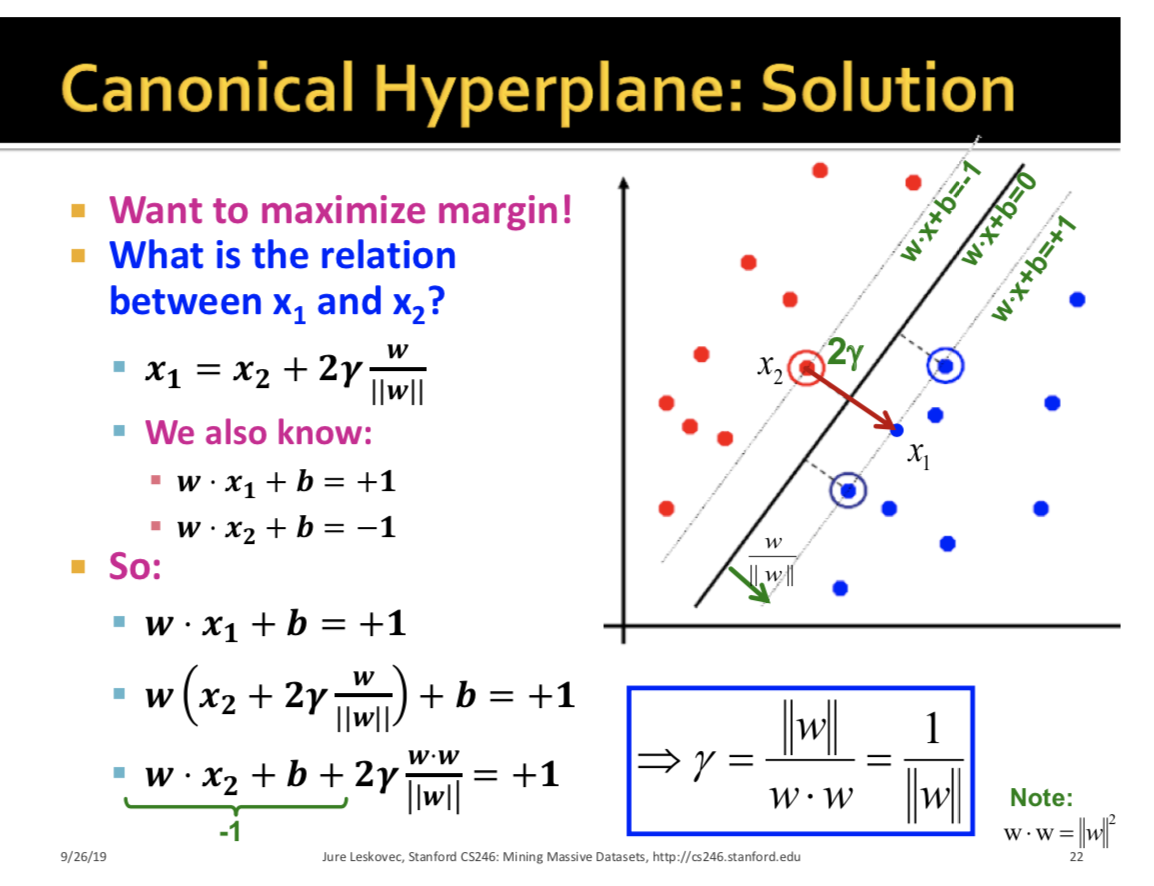
Given support vectors $x_1$, $x_2$, we have

• $x_1 = x_2 + 2m \frac{w}{

  w

  }$

• $w\cdot x_1 = +1$, $w\cdot x_2 = -1$, Therefore, $w(x_2 + 2 m \frac{w \cdot w}{||w||}) = +1$, and thus $-1 + 2 m \frac{w}{||w||} = +1 \rightarrow m= \frac{||w||}{w \cdot w} = \frac{1}{||w||}$ (Picture in 2)

$\max_{w} \frac{1}{||w||} \\ s.t. \forall i, y_i(\frac{w}{||w||} \cdot x_i ) \ge \frac{1}{||w||}$ (Eq 2)

And for the sake of training convenience, we change our objective function $\max_{w} \frac{1}{

w

}$ to $\min_w

w

$ to $\min_w \frac{1}{2}

w

^2$.

$\min_{w} \frac{1}{2}||w||^2 \\ s.t. \forall i, y_i(w \cdot x_i ) \ge 1$ (Eq 3 - SVM with Hard Constraints)

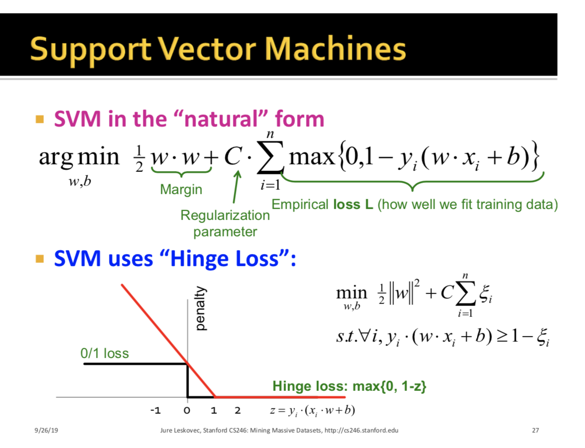
Next, we introduce slack variables $\zeta_i$ to allow for imperfect separability.

$\min_{w, \zeta_i \ge 0} \frac{1}{2}||w||^2 + C \cdot \sum_{i=1}^{n} \zeta_i \\ s.t. \forall i, y_i(w \cdot x_i ) \ge 1 - \zeta_i$ (Eq 4 - SVM with Slack Variables)

$\zeta_i$ is a penality term. If $x_i$ is on the wrong side of the margin, then get penalty $\zeta_i$. (If margin ≥ 1, don’t care, if margin < 1, pay linear penalty). We need to subtract the slack term from the constriants to make sure that they can still bind. $C$ is a regularization term: very large C means misclassified points are heavily penalized - we want close to perfect separability. C = 0 means that we can basically set $\zeta_i$ to anything and there is a very low penalty - this is too slack and basically ignores the data.

Finally, we rewrite the above in its hinge loss form: $\min_{w} \frac{1}{2}w \cdot w + C \cdot \sum_{i=1}^{n} \max \{0, 1-y_i(w \cdot x_i)\}$ (Eq 5 - SVM with Hinge Loss) Where each of the conditions $y_i (w \cdot x_i) \gt 1- \zeta_i$ became $\zeta_i \gt 1- y_i (w \cdot x_i)$, so it’s min value for each $i$ would be $1- y_i (w \cdot x_i)$ if the point was misclassified, or 0 if the point was correctly classified.

The corresponds perfectly to the hinge loss: (4)

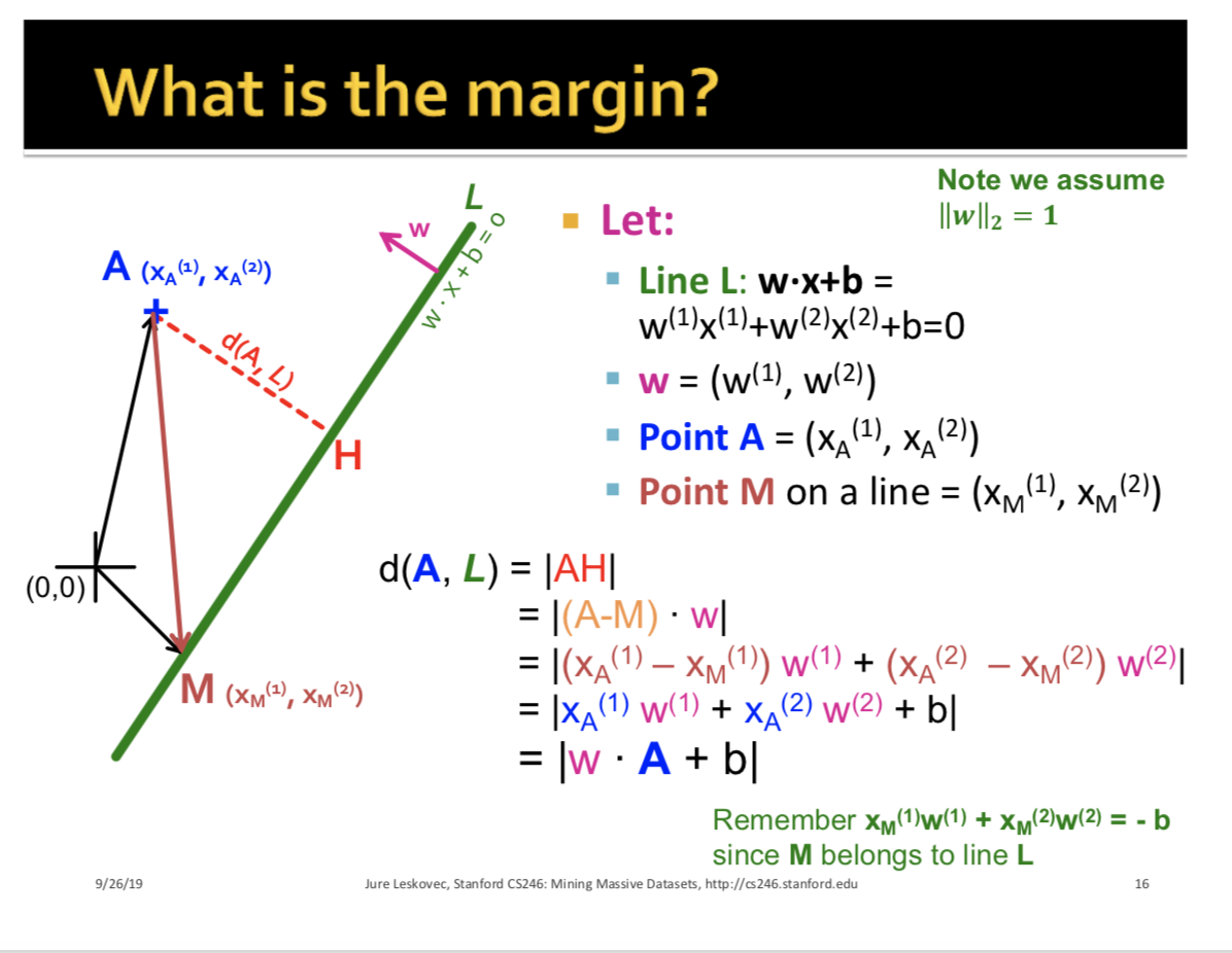
(0) There are generally $d+1$ support vectors for $d$ dimensional data. (1) This must be normalized so that we cannot arbitrarily scale $w$. (2) As in basic linear algebra, the value of $w \cdot x$ is the distance of the point $x$ to the line, with 0 being the separating line between negative and positive. Remember we one-pad $x$ in this notebook.

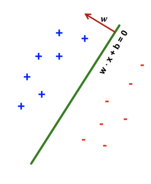
The margin is also the dot product $w \cdot x$ because the dot product is the projection of point $x$ onto the separating hyperplane orthogonal characteristic vector $w$.

(3) Note that $m$ is called $\gamma$ in the slides

(4) Hinge Loss