Ee261 lecture 8, 9, 10 scales, shifts and convolutions
1. Fourier Transforms of Transformed Functions
Delays (shifts in time) change the phase of the Fourier Transform: $Ff(s-b) = e^{-2 \pi i s b}Ff(s)$.
| Interpretation - shift in time corresponds to a phase shift in frequency, as the Fourier Transform is a complex number $Ff(s) = | Ff(s) | e^{2 \pi i \theta(s)}$, and thus $Ff(s-b) = e^{-2 \pi i s b}Ff(s) = | Ff(s) | e^{2 \pi i (\theta(s)-sb)}$. Here the magnitude of the spectrum didn’t change but the phase shifted. |
| Scaling (Stretching out of time) : $Ff(as) = \frac{1}{a} Ff(\frac{s}{a})$ if $a \ge 0$, $Ff(as) = -\frac{1}{a} Ff(\frac{s}{a})$ if $a < 0$. Written $Ff(as) = \frac{1}{ | a | } Ff(\frac{s}{a})$. |
| Interpretation - If $f(at)$ is a compressed version of $f(t)$, then $Ff(as) = \frac{1}{ | a | } Ff(\frac{s}{a})$ is stretched out horizontally (over the frequency domain) and shrunk in magnitude. If $f(at)$ is a stretched version of $f(t)$, then $Ff(as) = \frac{1}{ | a | } Ff(\frac{s}{a})$ is compressed out horizontally (over the frequency domain) and stretched in magnitude. |
You can’t have a signal which is localized in time and frequecy. If you localize a signal in time by squeezing it, you stretch out its spectrum in frequency.
Convolutions The field of Signal processig answers the question of how to use one signal to modify another. Usually, you are modifying the spectrum of a signal. When the modification we want is multiplucation of the spectra of two signals, that is given two signals $f$,$g$ to obtain $(Ff)(Fg)$ this is called convolution, written $(f * g)$.
\begin{align}
Fg(s) \cdot Ff(s) & = \left( \int_{-\infty}^\infty e^{2\pi i s t} f(t) dt \right) \left(\int_{-\infty}^\infty e^{2\pi i s x} g(x) dx\right)
& = \int_{-\infty}^\infty \int_{-\infty}^\infty e^{2\pi i s t} e^{2\pi i s x} g(x) f(t) dx dt
& = \int_{-\infty}^\infty \int_{-\infty}^\infty e^{2\pi i s (x+t)} g(x) f(t) dx dt
& = \int_{-\infty}^\infty \left( \int_{-\infty}^\infty e^{2\pi i s (x+t)} g(x) dx \right) f(t) dt
& = \int_{-\infty}^\infty \left( \int_{-\infty}^\infty e^{2\pi i s u} g(u-t) du \right) f(t) dt \;\; \text{; sub }u=t+x
& = \int_{-\infty}^\infty \left( \int_{-\infty}^\infty g(u-t) f(t) dt \right)e^{2\pi i s u} du \tag{1.1}
& = Fh(s)
\end{align}
where we define $h(u)$ as the convolution operator as below.
Def: The convolution of $f(t), g(u-t)$ as $h(u) = \int_{-\infty}^\infty g(u-t) f(t) dt$. We often write the convolution as $(f * g)(u)$ Then, (1.1) states that the convolution of $h(u)$, $Fh(s)$, is the product of the two signal frequencies $(Fg(s))(Ff(s))$.
Theorem: Given $f(t), g(u-t)$, and define the convolution of $f$ and $g$ as $h(u) = \int_{-\infty}^\infty g(u-t) f(t) dt$. Then, $F(f * g) = (Fg(s))(Ff(s))$.
Example of Convolution Use
Filtering is one of the main uses of convolution.
Suppose we had some data T about water clarity over time. The data has a lot of noise.
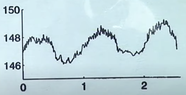
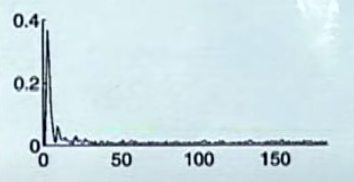
When we take the Fourier Transform, we see that the noise is caused by high frequencies in the spectra in the frequency domain. If we wanted to smooth the original function, we could kill off the high frequencies.
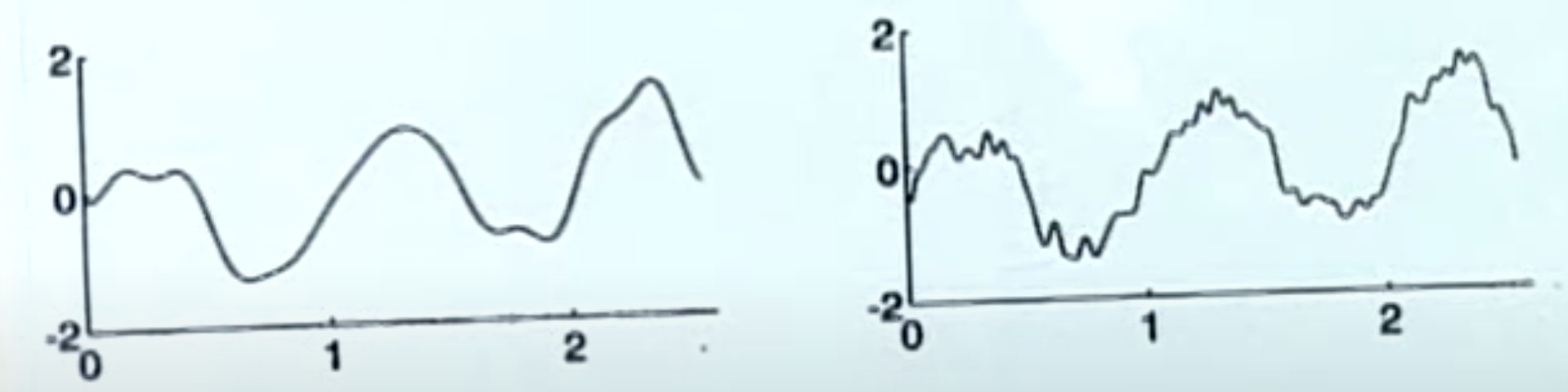
To kill off the high frequencies, we can multiply by a rectangle function π in the frequency domain (called a low pass filter). πFT(t) at thresholds (-v, v). The operation that achieves this in the time domain is the convolution ( 2v sinc(2vt) * T(t) ). The result here is to kill off the high frequencies. If you kill off all but the first 10 you get the graph to the left, if you kill off all but the first 40 you get the graph to the right.
2. More on Convolutions
Filters
A filter is a system that vonvolves a signal $f$ with a fixed signal $h$ (called an input response) ($g = (f * h)$). In the frequency domain, the spectrum is simply multiplied. $G(s) = F(s)H(s)$. To design a filter, is to design $H$.
Low pass filter - multiply by a scaled rectangle function from -v to v. Or, we can taper the signal slowly. High pass filter - multiply by a function which is 1 at high values and 0 in low values (1- rectangle function), to keep the high frequencies and drop the low frequencies. Used in traditional image processing for edge detection. Band pass filter - multiply by a shifted rectangle function.
In many cases, convolutions arises in cases of smoothing or averaging. The convolution of two functions is generally “smoother” than each function separately.
Facts:
- $\pi * \pi = \Lambda$ The convolution of the rectangle function with itself is the Triangle function.
- If $f$ is differentiable, and $g$ is not, $f * g$ is differentiable and $(f * g)’ = f’*g$. Similarly for higher derivatives.
- Derivative Theorem of Fourier Transforms: $(Ff’)(s) = 2 \pi i s Ff(s)$. The Fourier Transform of the derivative is $2 \pi i s$ times the fourier transform. Similarly, $(F(f^{(n)}))(s) = (2 \pi i s)^n Ff(s)$ The Fourier Transform turns differentiation into multipluation.
3. Example: Heat Equation
An infinte rod is heated up with initial temperature distribution $f(x)$. Temperature at time $t$ is $u(x,t)$. The heat distribution must satisfy the diffusion equation $u_t(x,t) = \frac{1}{2}u_{xx}(x,t)$ ($u_t$ is time derivative, $u_{xx}$ is spatial second derivative).
Take Fourier Transform of both sides of the diffusion equation. We handle the left hand side first. We take the Fourier Transform of $u_t$ in spatial variable $x$: $u_t(x,t) -> U(s,t)$. Then
\begin{align}
Fu_t(s, t) & = \int_{-\infty}^\infty e^{-2 \pi i s x} \frac{d}{dt} u(x,t) dx
& = \frac{d}{dt} \left( \int_{-\infty}^\infty e^{-2 \pi i s x} u(x,t) dx \right)
& = \frac{d}{dt} U(s,t)
\end{align}
We handle the right hand size, and use the Derivative Theorem (above) to obtain \begin{align} F(u_{xx})(s,t) = (2 \pi i s)^2 U(s,t) = -4 \pi^2 s^2 U(s,t) \end{align}
Equating the two sides, we obtain $\frac{d}{dt} U(s,t) = -4 \pi^2 s^2 U(s,t)$, and the solution to the differential equation is $U(s,t) = U(s,0) e^{-2 \pi^2 s^2 t}$. $U(s,0)$ is the Fourier transform of the inital distribution $u(x,0) = f(x)$. We denote this value $F(s)$. Thus, $U(s,t) = F(s) e^{-2 \pi^2 s^2 t}$.
The above equation gives that the Fourier Transform $U(s,t)$ is the product of two functions (The Fourier Transform of the initial distribution $F(s)$, and the Gaussian $e^{-2 \pi^2 s^2 t}$ Using (2.2), the solution of the heat equation is the original heat distribution convolved with a Gaussian.
COnvolution came up in this case because often to solve a differnetial equation we take a Fourier Transform, differentiation becomes multiplucation, and multiplucation in the frequency domain becomes convolution in the time domain.
(2.2) Using the fact that the Fourier Inverse of the Gaussian $e^{-2 \pi^2 s^2 t}$ is the Gaussian $\frac{1}{\sqrt{2 \pi t}}e^{- x^2 / (2t)}$. This is called the heat kernel.
4. Application of Convolution to the Central Limit Theorem
The CLT explains the universal appearence of the Gaussian curve in probability - Most probabilities in an average sense are distribution according to a Gaussian. For Fourier Transforms, $e^{- \pi x^2}$ is the “standard” Gaussian because its Fourier Transform is itself. In probability we use $\frac{1}{\sqrt{2 \pi}}e^{-x^2 / 2}$ because it has mean 0 and std dev 1.
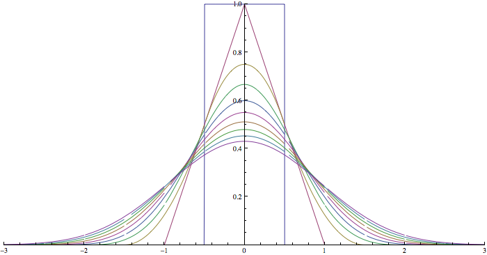
Recall that a convolution is something like a smoothing. Repeatedly applying the convolution operator to the rectangle function with itself makes it look more and more like a bell-shaped curve (first rectangle, then triangle, then smoother and smoother curves). This works with any function.
Given a random variable $X$ with pdf $p(x)$ and cdf between $a,b$ $\int_a^b p(x) dx$, we have Theorem: Convolutions of Probability Distributions: If $X_1$ and $X_2$ are independetn random variables with distributions $p_1(x), p_2(x)$, then the distribution of $X_1 + X_2$ is given by the convolution $p_1 * p_2$. (The distribution of the sum of two random variables is the convolution of their distributions).
Proof: For any value of $t$, $P(X_1+X_2 \le t) = \int \int_{x_1+x_2 \le t} p_1(x_1) p_2(x_2) dx_1 dx_2$. Make a change of variable in the integral $x_1 = u, x_2 = v-u$
\begin{align}
P(X_1+X_2 \le t) & = \int \int_{x_1+x_2 \le t} p_1(x_1) p_2(x_2) dx_1 dx_2
& = \int_{-\infty}^{\infty} \int_{-\infty}^{t} p_1(u) p_2(v-u) du dv \;\; \text{change of variables (4.1)}
& = \int_{-\infty}^{t} \left( \int_{-\infty}^{\infty}p_1(u) p_2(v-u) du \right) dv \;\;
& = \int_{-\infty}^{t} (p_1 * p_2)(v) dv
\end{align}
Since $P(X_1+X_2 \le t) = \int_{-\infty}^{t} (p_1 * p_2)(v) dv$, $(p_1 * p_2)$ is the pdf of the random variable corresopnding to $X_1+X_2$.
Corollary: The pdf of the distribution $X_1 + X_2 + \cdots + X_n$ is $p_1 * p_2 * \cdots p_n$.
(4.1) Note that the change of variables in this case also requires multiplying by the norm of a Jacobian, but this is 1 all around in this case.
The Central Limit Theorem: Suppose $X_1, …, X_n$ are $n$ independent iid random variables, each with distribution $p(x)$ with mean 0 and stddev 1.Then $X_n = X_1 + X_2 + \cdots + X_n$ has mean 0 and stddev $\sqrt{n}$. We tend to use $\frac{X_n}{\sqrt{n}} = \frac{ X_1 + X_2 + \cdots + X_n}{\sqrt{n}}$ which has mean 0 and stddev 1. Then, as $n \to \infty$, $P(a \le \frac{X_n}{\sqrt{n}} \le b) \to \frac{1}{\sqrt{2 \pi}} \int_a^b e^{-x^2/2}$.
Proof: We show that if $p_n(x)$ is the pdf of $\frac{X_1 + X_2 + \cdots + X_n}{\sqrt{n}}$, then as $n \to \infty$, $p_n(x) \to \frac{1}{\sqrt{2 \pi}} e^{-x^2/2}$. By the above, we have the distribution of $X_1 + X_2 + \cdots + X_n$ is $\underbrace{(p * p \cdots * p)}{n \text{ times}}(x)$. We use the fact that the distribution of the scaled version, $p_n(x) = \sqrt{n}\underbrace{(p * p \cdots * p)}{n \text{ times}}(\sqrt{n} x)$. Below, we denote $\underbrace{(p * p \cdots * p)}_{n \text{ times}}(x)$ as $p^{*n}(x)$.
We take the Fourier Transform, and turn convolution to multiplication:
\begin{align}
F(p_n(x)) & = \sqrt{n} F( p^{n}(\sqrt{n} x))
& = \sqrt{n} \frac{1}{\sqrt{n}}(Fp^{n})(\frac{s}{\sqrt{n}}) \;\; & \text{Using the scaling theorem}
& = [(Fp)(\frac{s}{\sqrt{n}})]^n \;\; & \text{Convolutions cause their Fourier Transforms to be multiplied }
\end{align}
Now we use the Taylor Series for Complex Exponentials to expand the exponential term in the Fourier equation:
\begin{align}
(Fp)(\frac{s}{\sqrt{n}}) & = \int_{-\infty}^{\infty} e^{-2 \pi i (s/\sqrt{n}) x} p(x) dx
& = \int_{-\infty}^{\infty} \left[ 1 - \frac{2 \pi i s x}{\sqrt{n}} - \frac{1}{2}\left( \frac{2 \pi s x}{\sqrt{n}} \right) ^2 + \cdots \right] p(x) dx
& = \left[\underbrace{ \int_{-\infty}^{\infty} p(x) dx }{=1 \text{ p(x) is prb dist}}\right]
- \left[ \frac{2 \pi i s}{\sqrt{n}} \underbrace{\int{-\infty}^{\infty} xp(x) dx }{=0 \text{ is mean}}\right]
- \left[ \frac{1}{2}\left( \frac{2 \pi s}{\sqrt{n}} \right) ^2 \underbrace{ \int{-\infty}^{\infty} x^2 p(x) dx}_{=1 \text{ is std dev}}\right]
+ \cdots
& = 1 + 0 + \frac{2 \pi^2 s^2}{n} + \cdots
(Fp)(\frac{s}{\sqrt{n}}) & \approx 1 + \frac{2 \pi^2 s^2}{n}, \text{ so,}
F(p_n(x)) = [(Fp)(\frac{s}{\sqrt{n}})]^n & \approx \left( 1 + \frac{2 \pi^2 s^2}{n}\right)^n \xrightarrow{n\rightarrow\infty} e^{-2\pi^2s^2}
\end{align}
Since $[(Fp)(\frac{s}{\sqrt{n}})]^n = F(p_n(x))$ is the Fourier Transform of the distribution function, we take the inverse Fourier Transform to both sides to recover the distribution. But above, we have that the Inverse Fourier Transform of the Gaussian $e^{-2\pi^2s^2}$ is $\frac{1}{\sqrt{2 \pi}} \int_a^b e^{-x^2/2}$, the standard normalized Gaussian, and we are done.