Cs224n lecture 13 bert, contextual word embeddings, pretraining

18 April 2020 - 14 mins read time

Reflections on Word Representations (“The most exciting thing in NLP and Deep Learning in 2018”)

Word Representations

Pre-trained word vectors was really the secret sauce getting NN to work in NLP in 2011.

In most cases, pretrained word vectors helps a lot over random word vectors becuse we can train them on much more data.

These have two problems with traditional word representations like Word2Vec, GloVe, FastText:

• Words have a lot of senses and you are collapsing all of those together.
  • What we really want to know is very fine-grained word sense disambguation in its context of use.
• We just have one representation for a word, but words have different aspects, including semantics, syntactic behavior, and register/connotations.

Pre-ELMo - TagLM (Semi-Supervised Learning)

Peters et al 2017

Idea: Want meaning of word in context, but standardly learn task RNN only on small task-labeled data (ie NER)

Why don’t we do semi-supervised approach where we train NLM on large unlabeled corpus, rather than just word vectors.

We start off with a ton of unlabeled data.

1. Pre-train both a conventional word embedding model like word2vec as well as a bi-LSTM langauge model. After pre-training, freeze the bi-LSTM so it is not updated in model updates.

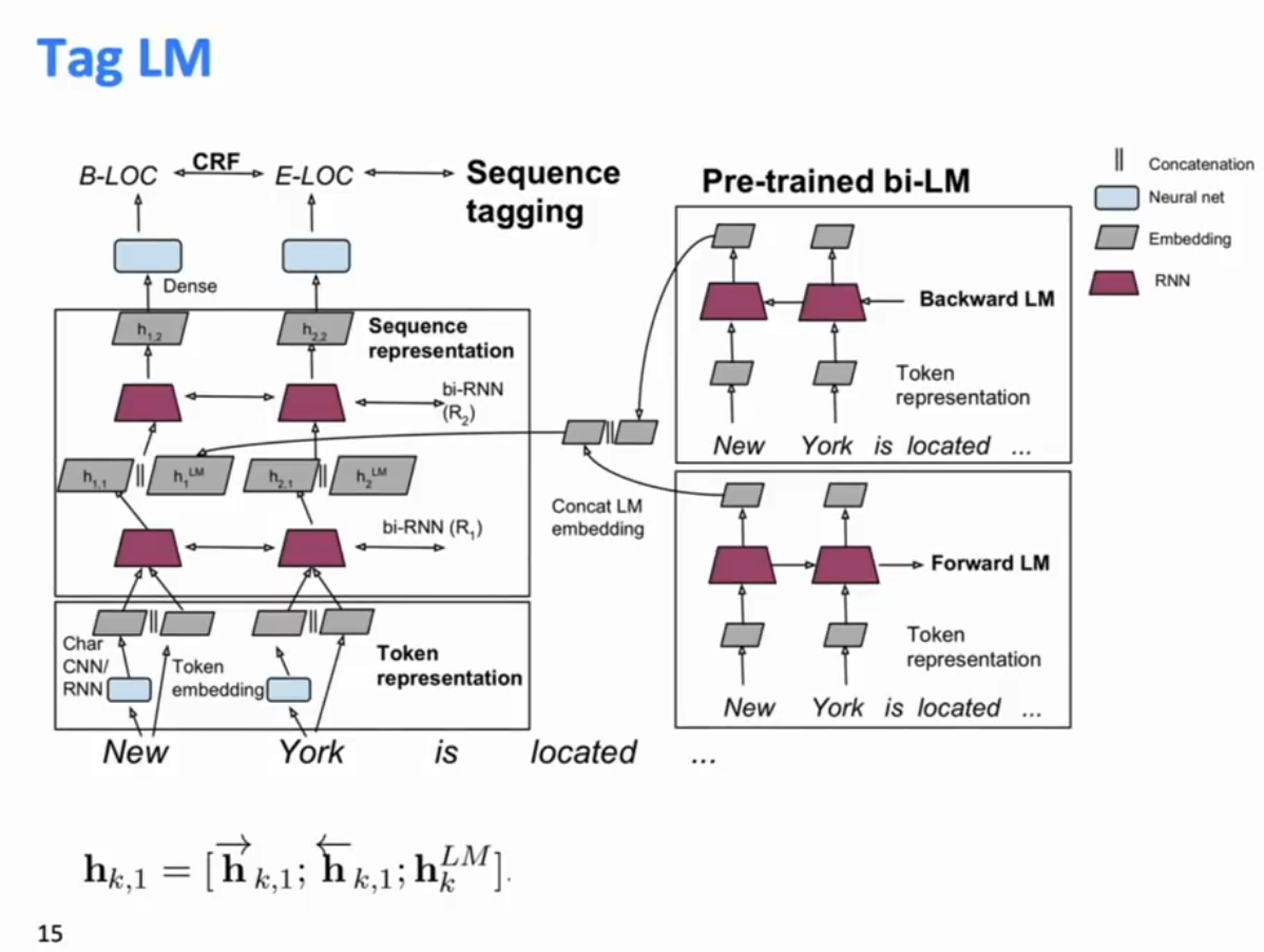
2. Then when we want to learn our supervised POS tagging, for the input words we not only use the word embedding which is context independent, but we also use the bi-LSTM language model hidden state at the input, and we feed both in as features in our sequence tagging model.

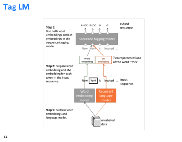
Their full model is below (in the full model they also use a character level language model to do embeddings, and the piucture below show how they contatenate hidden states to get their output.)

‘

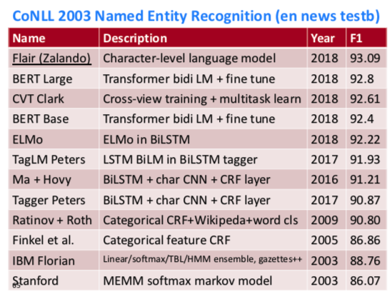
They got SOTA in Named Entity Recognition. in 2017

• Proved that Contextual Word Representations really had some power and were useful.

Some details:

• Language model is trained on 800 million traning words of ‘billion word benchmark’
• A LM trained on supervised data does not help.
• Having a huge LM design helps over a smaller model
• Using just LM embeddings to predict isn’t great: 88.17 F1.

ELMo Embeddings from Language Models NAACL 2018

Peters et al 2018.

The breakthrough paper for contextual word vectors (more precicely word token vectors). Proved that everyone should be using them, and should not be using traditional word vectors.

ELMO learns word token vectors using long context (here, whole sentence), not context windows. Learn a deep bi-LSTM and use all its layers in prediction.

Architecture was actually very similar to TagLM and by the same authors, but they modified it to make it better.

The trained a bidirectional LM. The aim was a performant but not overly large LM.

• Use 2 biLSTM layers
• Use character CNN to build initial word representation (only), no word-level representation (This lessens the number of parameters you have to store)
  • They use 2048 char n-gram filters and 2 highway layers, 512 dim projection.
• The expanded the dim of the LSTM hidden/cell states to 4096 but projected down to 512 dimensions (with a feedforward projection layer) to next input. [This is a common trick to reduce the dimensionality of the input]
• Use a residual connection
• Tie parameters of token input and output (softmax) and tie these between forward and backward LMs.

Instead of doing, as in common practice then and in TagLM, just using the top layer of the bi-LSTM stack as input to the task-specific prediction model, ELMO uses the hidden state at all the layers of the neural LN in combination. That is, ELMO learned task-specific combinations of bi-LM representations. This is an inovation that imporves on just using top layer of LSTM stack.

That is, if inputs and the hidden layers states of the bi-LSTM layers $j=1,…,L$ are $R_k$as below: \begin{align} R_k = & { x_k^{LM}, \overrightarrow h_{k,j}^{LM}, \overleftarrow h^{LM}{k,j} | \; j= 1,…,L }
= & { h^{LM}{k,j} | \; j= 1,…,L } \end{align} Then $ELMO_k^{task} = E(R_k ; \Theta^{task}) = \gamma^{task} \sum_{j=1}^L s_j^{task} h^{LM}_{k,j}$ where

• $y^{task}$ scales overall global usefulness of ELMO to the task in question.
• $s^{task}$ are softmax-normalized mixture model weights. It is a learned weight applied to any particular level in the bi-LSTM.

Use of ELMO with a Task

• First run bi-LM to get representaions for each word
• Then let (whatever) end-task model use them.
  • Freeze weights of ELMO for purposes of using them in a supervised model
  • You can then use the representaitons however you want. The recommended way is to concatenate ELMO weights into the representation of a particular word in some task-specific model (The details of course depend on the task; often concatenating into intermediate layer as for TagLM is typical.) Example in pic below.
  • The supervised model can also be trained to predict ELMO representaitons again when producing outputs, such as in a QA system.

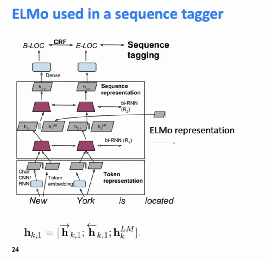
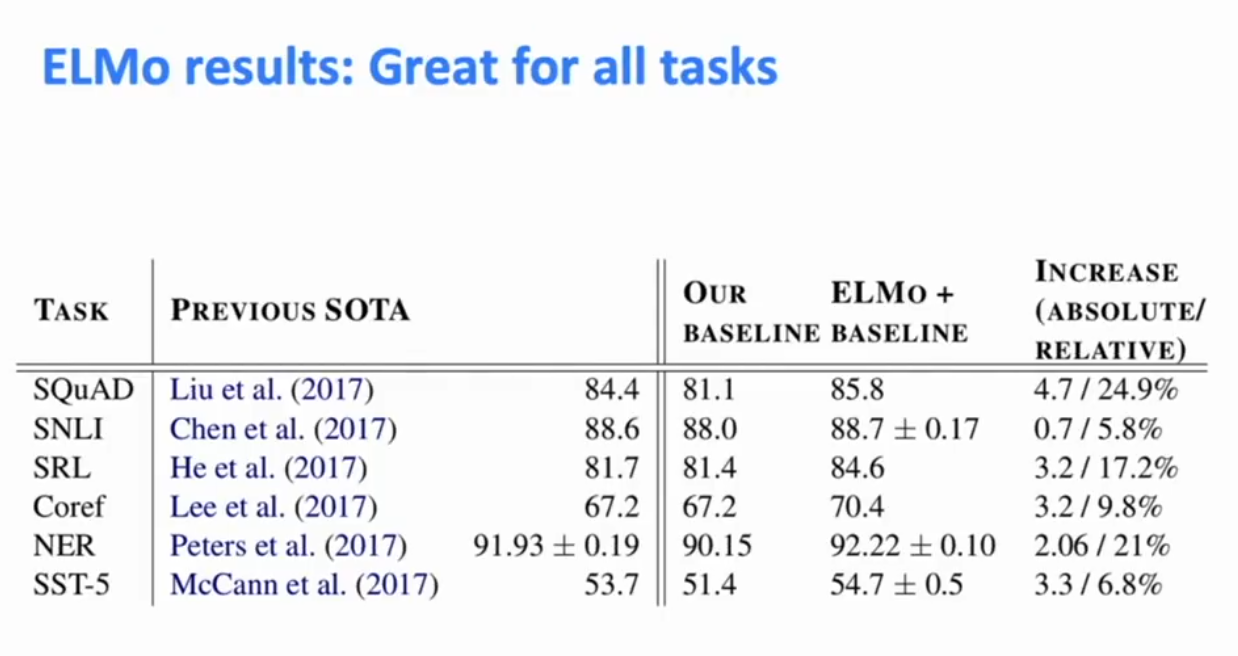
ELMO representations can be used for any NLP task and gives gain across the board!

ELMO: Weighting of Layers

The two bi-LSTM LM layers have differentiated uses/meanings

• Lower layer(s) is better for lower-level syntax, etc.
  • POS tagging, syntactic dependencies, NER
• Higher layer(s) is better for higher level semantics
  • Sentiment, Semantic role labelling, QA, SNLI

What if we had ELMO with more layers?

** **

ULMfit (Fast.ai) 2018

Fine Tuning

Universal Langauge Model Fine-Tuning for Text Classification. Howard and Ruder (2018)

Same general idea of transferring NLM knowledge, learn a big language model first, and then apply it to various tasks. The task they tested here was text classification,m

Idea: Gradually fine-tuning.

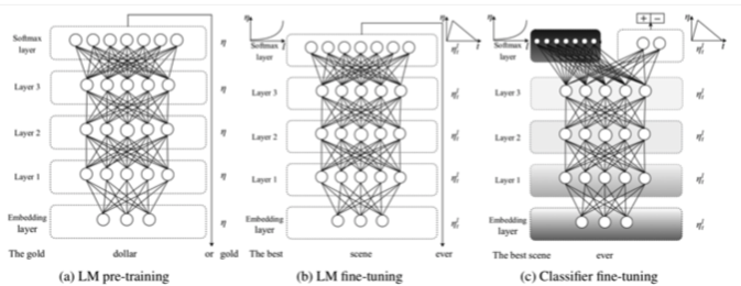
Fine-Tuning Process:

Use a big unsupervised corpus to train a big neural language model.

Fine tune LM on target-domain task data.

Fine tune as classifier on target task. Remove the top layer and replace with a classifier softmax, using your fine-tuned LM.

Use reasonable-size “1 GPU-day” model, which is not super huge.

Used a lot of details about fine-tuning to maximize performance

• (Differnet per-layer learnign rates, slanted triangular learning rate STLR schedule)

• Gradual layer unfreezing and STLR when learning classifier

• Classify using concatenation [hT, maxpool(h), meanpool(h)]

** **

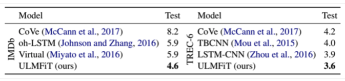
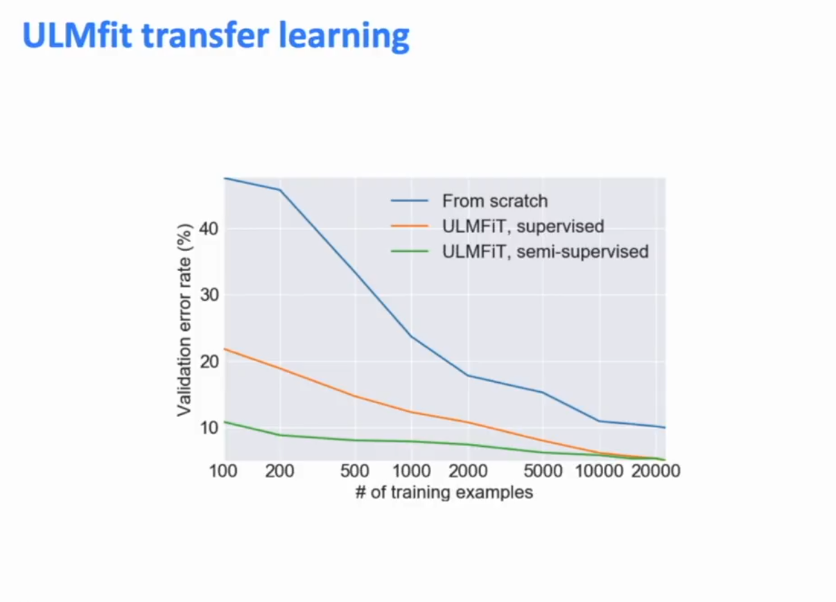
They were able to significantly improve on SOTA (Results in Appendix 2). Also, if you already trained the neural LM on a big amount of data, you are able to do well on your supervised task even when trained on very little data. (Appendix 3)

Current (2020) SOTA Systems for Language Modelling

The current (2020) SOTA systems for langauge modeling have just taking contextual embeddings ala ELMO and fine-tuning and have scaled it up enormously.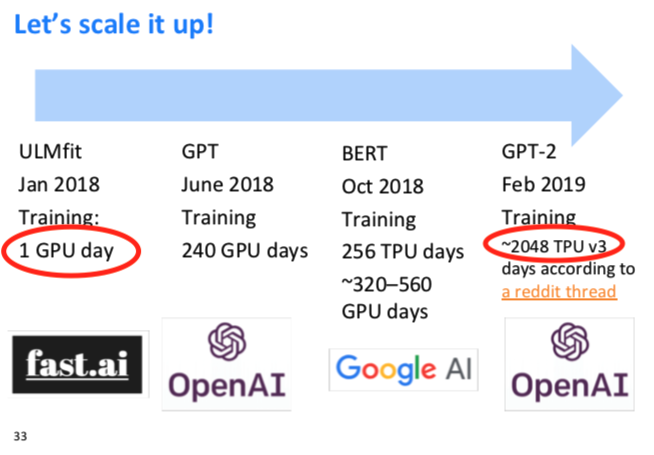

** **

Transformers

Attention is all you need (2017), Aswani, Shazeer et al.

Idea: We want parallelization but RNNs are inherently sequential. Despite GRUs and LSTMs, RNNs still need attention mechaism to deal with long range dependencies - path length between states growth with sequence otherwise.

But if attention gives us access to any state, maybe we can just use attention and don’t need the RNN?

Recommended resource to learn about Transformers:

[The Annotated Transformer by Sasha Rush] (http://nlp.seas.harvard.edu/2018/04/03/attention.html)

A Jupyter Notebook using PyTorch that explains everything!

Dot Product Attention

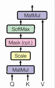
Inputs: A query $q$ and a set of key-value (k-v) pairs to an output. Query, key, values and output are all vectors. Ourput is weighted sum of values, where the weight of each value is computed by a dot product of query and corresopnding key, and looking up the weighting for each corresponding value. Queries and keys have the same dimensionality $d_k$ and value has dimensionality $d_v$.

$A(q,K,V) = \sum_i \frac{e^{q \cdot k_i}}{\sum_j e^{q \cdot k_j}} v_i$ In matrix form, this is $A(Q,K,V)=softmax(QK^T)V$

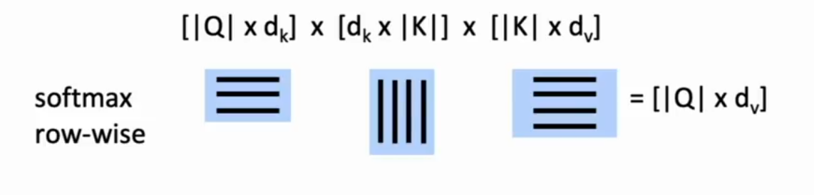
The attention score is the weighted sum of the values weighted by the attention score, which squashes all the individula reprenstations into one. Scaled Dot-Product Attention

Problem: As $d_k$ gets large, the variance of $q^Tk$ increases, so some values inside the softmax gets large, so the softmax gets incredibly peaked, and its graident gets smaller. Solution: Scale by length of query/key vectors: (Pic in Appendix 4) $A(Q,K,V) = softmax \left(\frac{QK^T}{\sqrt{d_k}}\right)V$

Self-Attention in the Encoder

In the encoder, everything in the attention input is our word vectors: the queries, keys and values are all our word vectors. In other words, the word vectors themselves select each other.

We’ll see in the decoder why we separate them in the definition.

Multi-head Attention

Problem with simple self-attention: Only one way for words to interact with one another. Maybe we wnat multiple types of attention, some to capture syntax, some semantics, some other dependencies.

Solution: Multi-head attention

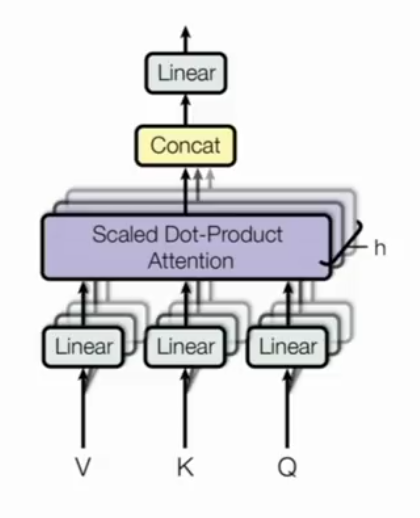
First map Q, K, V into h=8 many lower dimensional spaces via W matrices. Then apply attention, then concatenate ourputs and pipe through linear layer. (Picture in Appendix 4) \begin{align} MultiHead(Q,K,V) = & \; Concat(head_1,…,head_h)W^O
\text{where } head_i = &\; Attention(QW_i^Q, KW_i^K, VW_i^V) \end{align} The multi-head attention was one of the successful innovations that made the transformer a successful architecture.

Complete Transformer Block

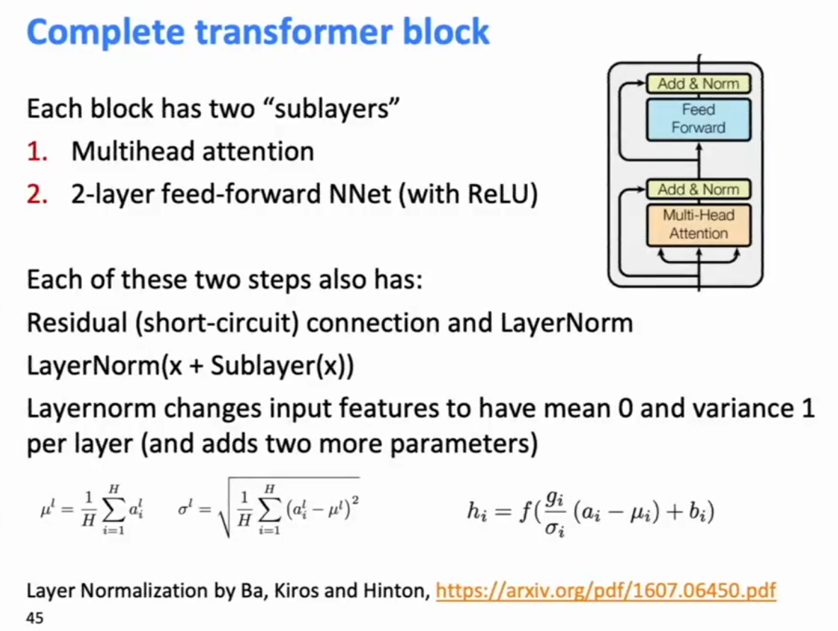
There’s no free lunch. You now no longer have recurrent informaiton carried along a sequence. You’ve got a word at some position which can be casting attention on other words, so if you like to have information carried along the chain, you ahve to walk the first step of the chain, and then you need to have another lauer that walks another step of the chain. So you’re getting rid of the recurrence but you’re substituting some depth to allow thigns to walk along multiple hops. But nevertheless, that is highly advantageous in GPU architectures which can compute everything at once.

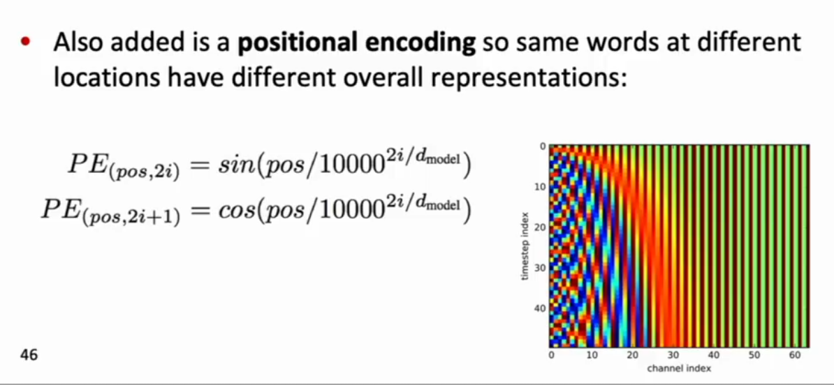
Positional Encoding

Note that their actual word representaitons are byte-pair encodings.

Complete Transformer Encoder

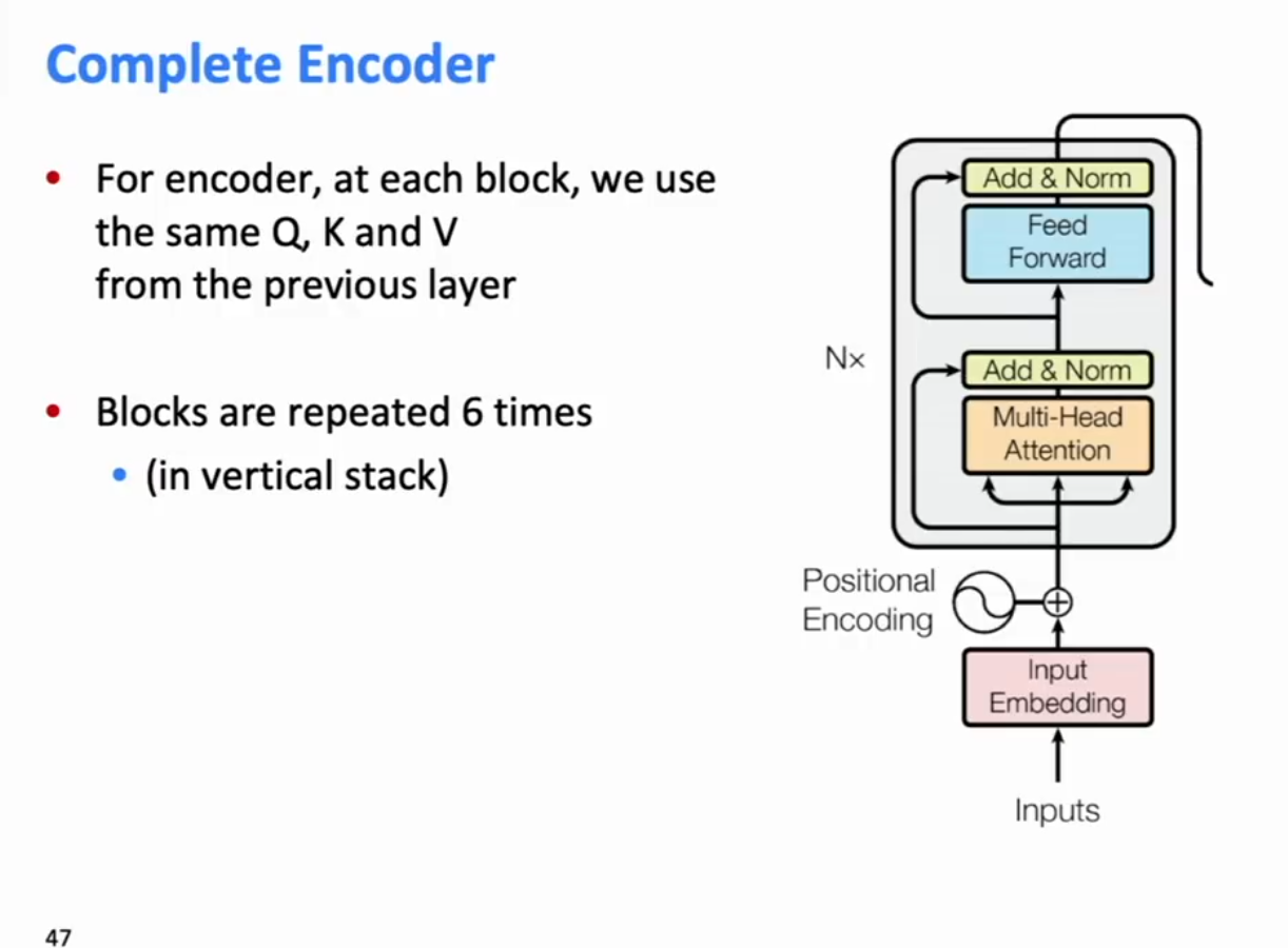
Interpretation: At each stage you can look with multi-headed attention at various places in the sentence, accumulate information, push it up to the next layer, and if you do that 6 times, you can be starting to progressively push information along the sequence in either direction to calculate values that are of interest.

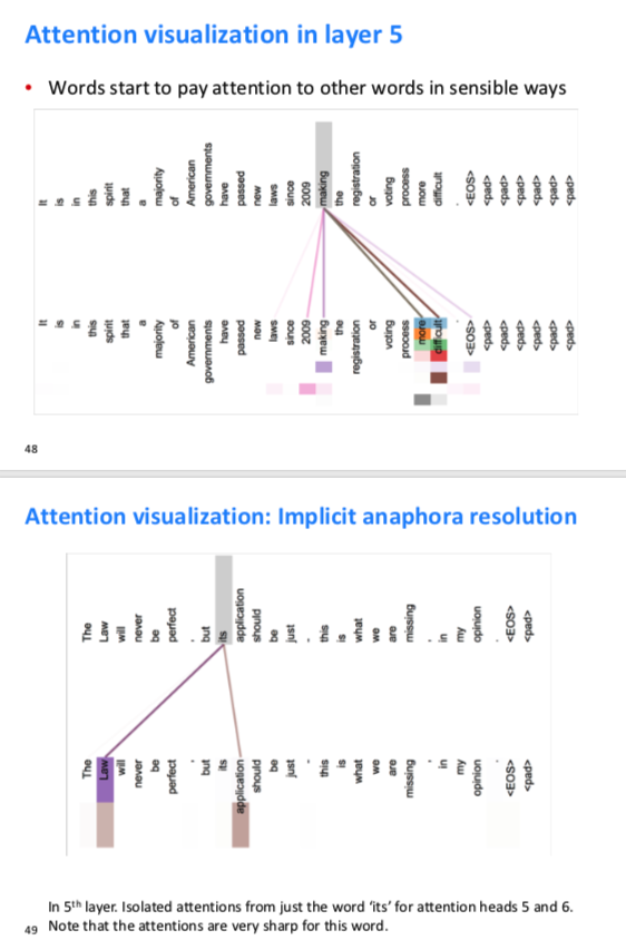
The attention heads attend to each other in interprable ways, and can correspond to modifiers of the word, close by words, or anaphora resolution. (Appendix 6)

Transformer Decoder

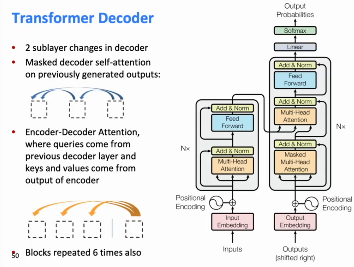
Decoderat level n is attending to the encoder hidden state at level n (or the top level of the encoder?), not to itself (the decoder module is not using self-attention)

BERT: Bidirectional ENcoder Representaitons from **Transformers 2018.**

Devlin, Chang, Lee Toutanova 2018.

Pre-training of Deep Birectional Transformers for Language Understanding

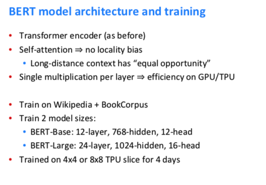
Uses an encoder for a transformer network to calculate a representation of a sentence, to use as an all-purpose representation of a sentence for all tasks.

Problem: Langage models only use left or right context, but languge understanding is bi-drectional.

Why are LMs unidirectional?

• Reason 1: Directionality is neede to generate a well-formed probabilty distribution (we dont care about htis)
• Reason 2: Words cna ‘see themselves” in a bidirectional encoder.

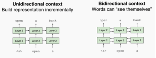
How do you get bi-directional context without words being able to see themselves?

Solution: Train things with a Transformer Encoder, and then train on a language model-like objective: no longer predicting the next word moving left to right, but “fill-in-the-blank”:

Mask out k% (k=15%) of the input words, and then predict the masked words.

the man went to the [MASK]{store} to buy a [MASK]{gallon} of milk

Masking is a tradeoff. Too little masking: Too expensive to train. Too much masking: Not enough context.

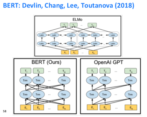
They argue that OpenAI’s GPT is a classic langauge model working left to right, so you only get left context, for the ELMO langauge model, it’s two separate langauge models: a right-to-left language model and a left-to-right language model, but BERT jointly uses context from both sides at all times.

BERT Complication: Next Sentence Prediction:

(Less Improtant) BERT wanted to make their language model coherent across sentences and able to preserve meaning from sentence to sentence. This makes it useful for QA systems and other systems that ask about meaning over sentences (and not just whether the right words probabilistically follow the ones around it), so in addition to their fill-in-the-blank loss funciton they also had a secondary loss function who’s purpose was to learn relationships between sentences.

Given two sentences, predict whether Sentence B is actual sentence that proceeds Sentence A or a random sentence. ALso train a loss based on the next sentence prediction task.

What did BERT use for embedding?

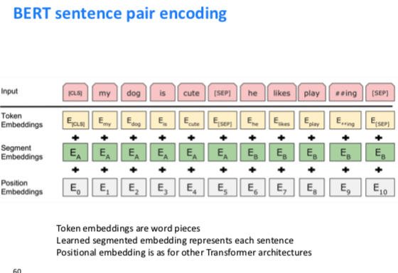
BERT used a standard token embedding over BPE tokens (as in other langauge models) plus (not concatenate!) a position embedding (as in other position embeddings) plus segment embeddings telling whether the word appears in teh first sentence or the second sentence.

These three things added togehter become the token representations for each pair of sentences. These are put into a transformer model where you have losses when you cannot predict the masked words or if you misclassify the second sentence as correct or not.

** **

** **

Fine-Tuning Training and then Using BERT in Various Tasks

You can take the BERT language model pre-trained, and you can use it for a large number of different tasks** **by taking off the top level prediction model, use the hidden state representations of each word in context generated by BERT, and then fine tune it on training data for a particular task.

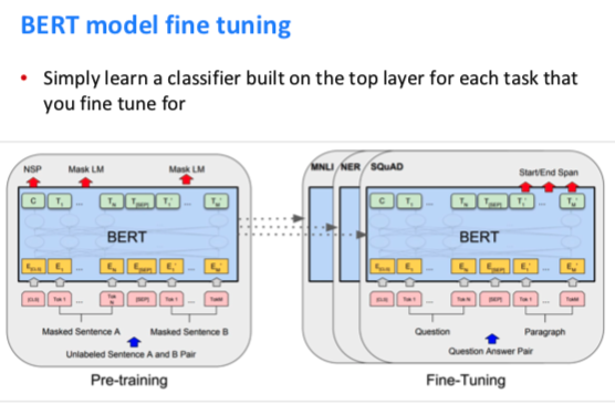
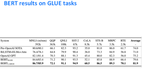
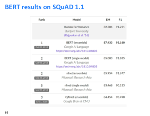
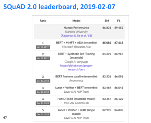
BERT has performed amazingly on almost all NLP tasks. The results are in Appendix 7.

Current State of NLP

We now have strongly performing, very deep, pre-trained neural network stacks, for NLP in the same way vision has had for 5 years (ResNet, etc)! Now to do NLP, you want to be using deep pretrained transfomer stacks to get the best performace.

If you’re interested in Machine Learning, there’s no shortage of interesting problems to work on!

Appendix

(1)

Dealing with <unk>s

a) if the <unk> word at test time appears in your unsupervised word embeddings, just use the vector from your pretrained word embeddings as is at test time.

b) additionally, for other words, just assign them a random vector, adding them to your vocabulary.

(2) Results of ULMfit performance.

(3)

(4)

Appendix 6: Interpretation of Attention in Transformer

** **

Appendix 7: BERT Results

BERT results on GLUE (Natural Language Inference) tasks, which are defined in Appendix 8.

The point of BERTBASE is to have a model about the same size as previous ones for the point of comparison, and the point of BERTLARGE is to show that you can get even better results by going with an even larger model.

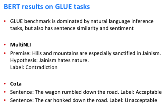
Appendix 8: Natural Langauge Inference (GLUE) tasks.