Cs224n lecture 11 cnns for nlp
Learn about how to debug neural nets
CNNs and Downsides of RNNs:
RNNs cannot capture phrases without prefix context
Often capture too much of last words in final vector.
CNNs are very fast! Much faster than RNNs
CNNs
What if we conpute vectors for every possible word subsequence of a certain length? (Every n-gram)
Convolutions
A patch or kernel of weights which is slid over a sequence (or matrix), producing a dot product for each position. When we run CNNs we often pad the front and back so the ourput is the same length.
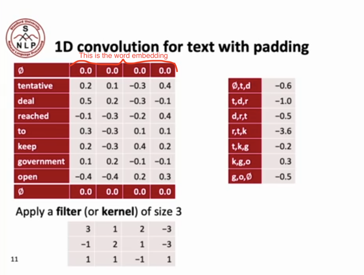
Because one convolution only captures one value for each filter, we often use multiple filters to get multiple values, which we call features. The idea is that each filter specializes in some aspect of the sentence.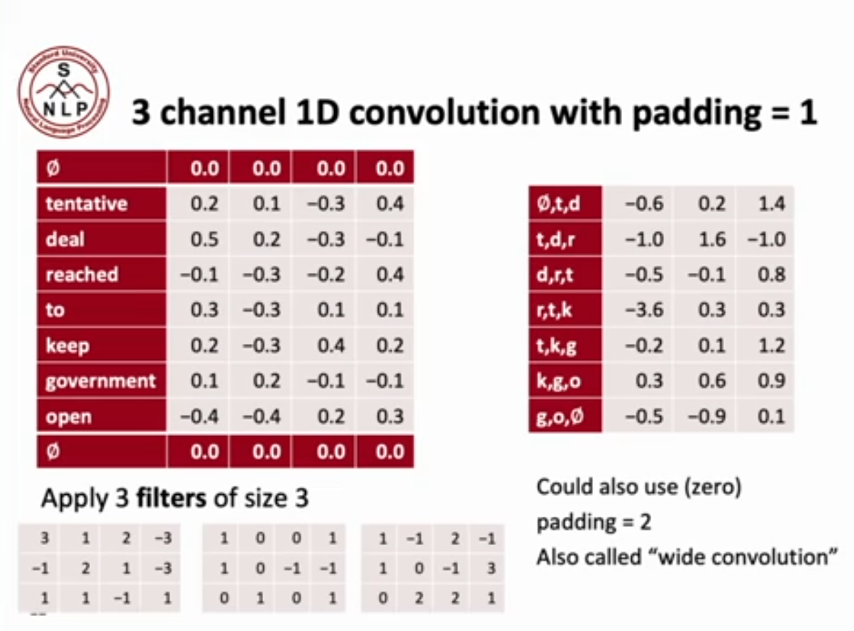
Important Ideas for CNNs (With NLP Focus)
Maxpooling
Summarizes the output of a CNN.
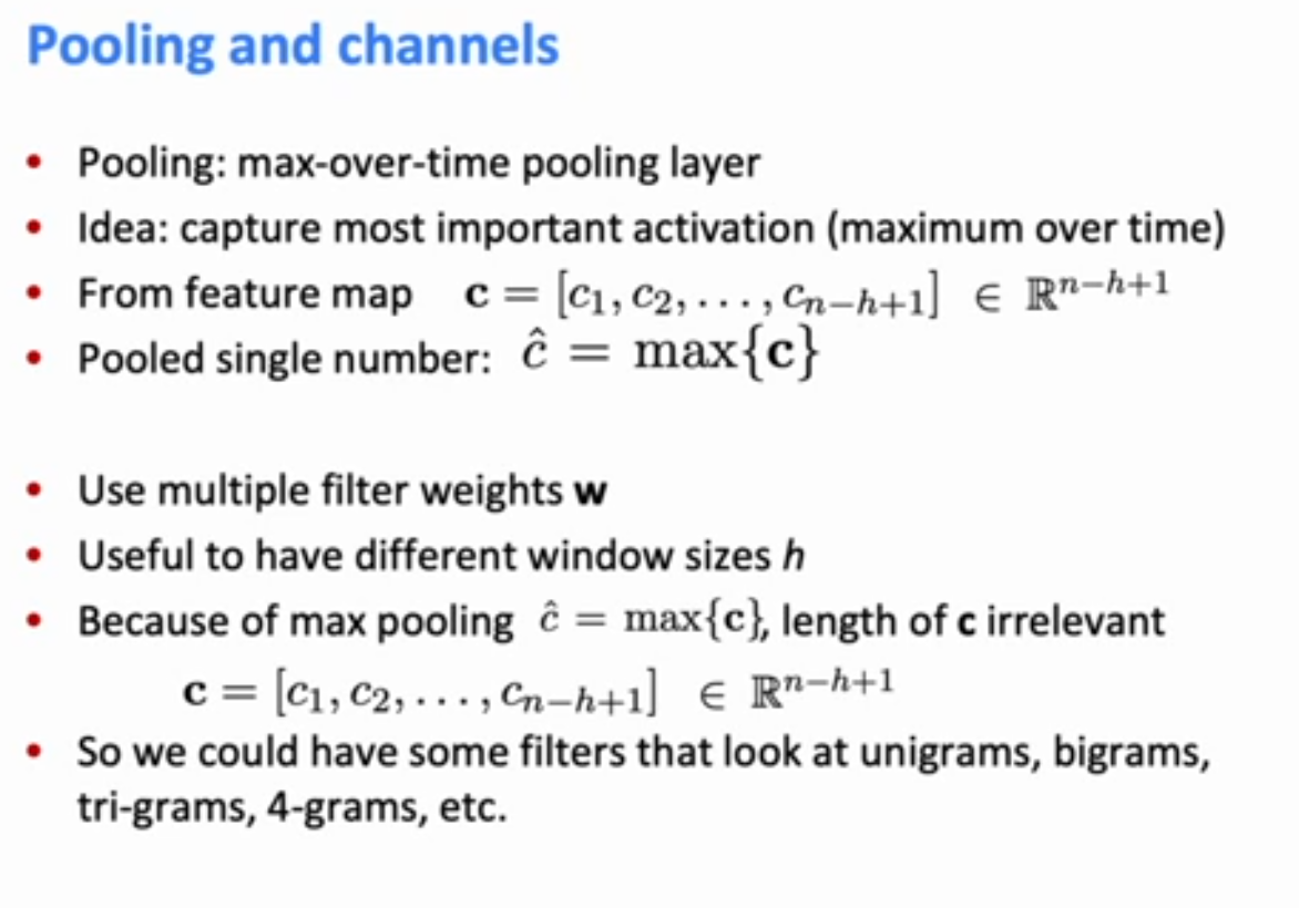
For each of the features computed by the convolution, compute the max over all words of the returned feature values.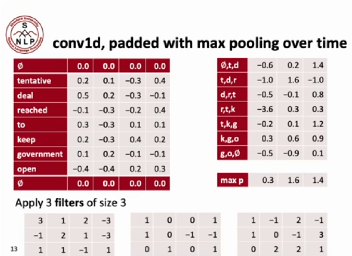
Batch Norm
(Ioffe and Szegedy. 2015.)
Batch norm is almost always used in deep CNNs.
Transform the convolution output of a mini batch (whatever random 32 examples you saw) by scaling the activations to have zero mean and unit variance before pushing it to the next layer of the Conv Block. Ensures that what comes out of the conv block are always at the same scale.
- This allows deep NNs to learn much more reliably, becasue a lot of hyperparameter tuning in deep NN training is being very fussy about hyperparaneters to keep a scale of things about right so they dont get too big or too small. Batch-norm takes away the need to be so fussy about it.
1x1 Convolutions
1x1 Convolutions are convolutions with a kernel size of 1. This gives you a position specific fully connected linear layer across channels!
You can do this because you want to map down from having a lot of channels to having fewer channels, or to get another linearities.
If you put fully connected layers over everything, they involve a lot of parameters, but putting in size 1 convolutions involve very few parameters.
Avg pooling
You can also take the average of each computed feature for each value. This corresponds roughly to “on average how much of this feature, ie. the sentence being about food, is present in the sentence?” Sometimes used. Used much less than maxpool.
Other Notions
Other notions used in CNNs but less common in NLP applications are in Appendix (2). They include
- Stride(2), Local Max Pool, Stride=2, k-max pooling over time
Convolutional Neural Networks for Sentence Classification (2014, very early paper)
Single Sentence Text Classification (Old)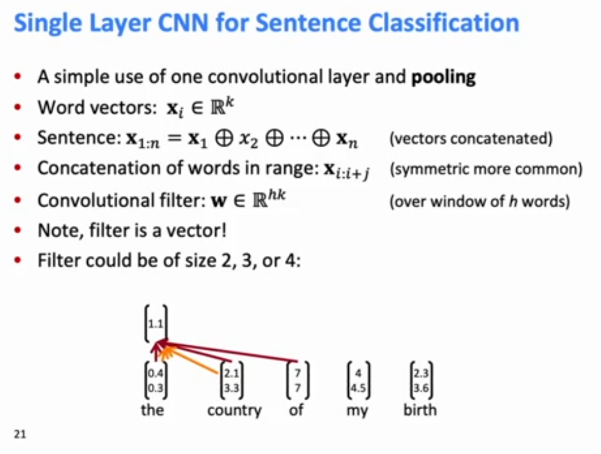
Below, f is a nonlinearity. In this paper they use a bias term and right-padding only (most people do symmetric padding).
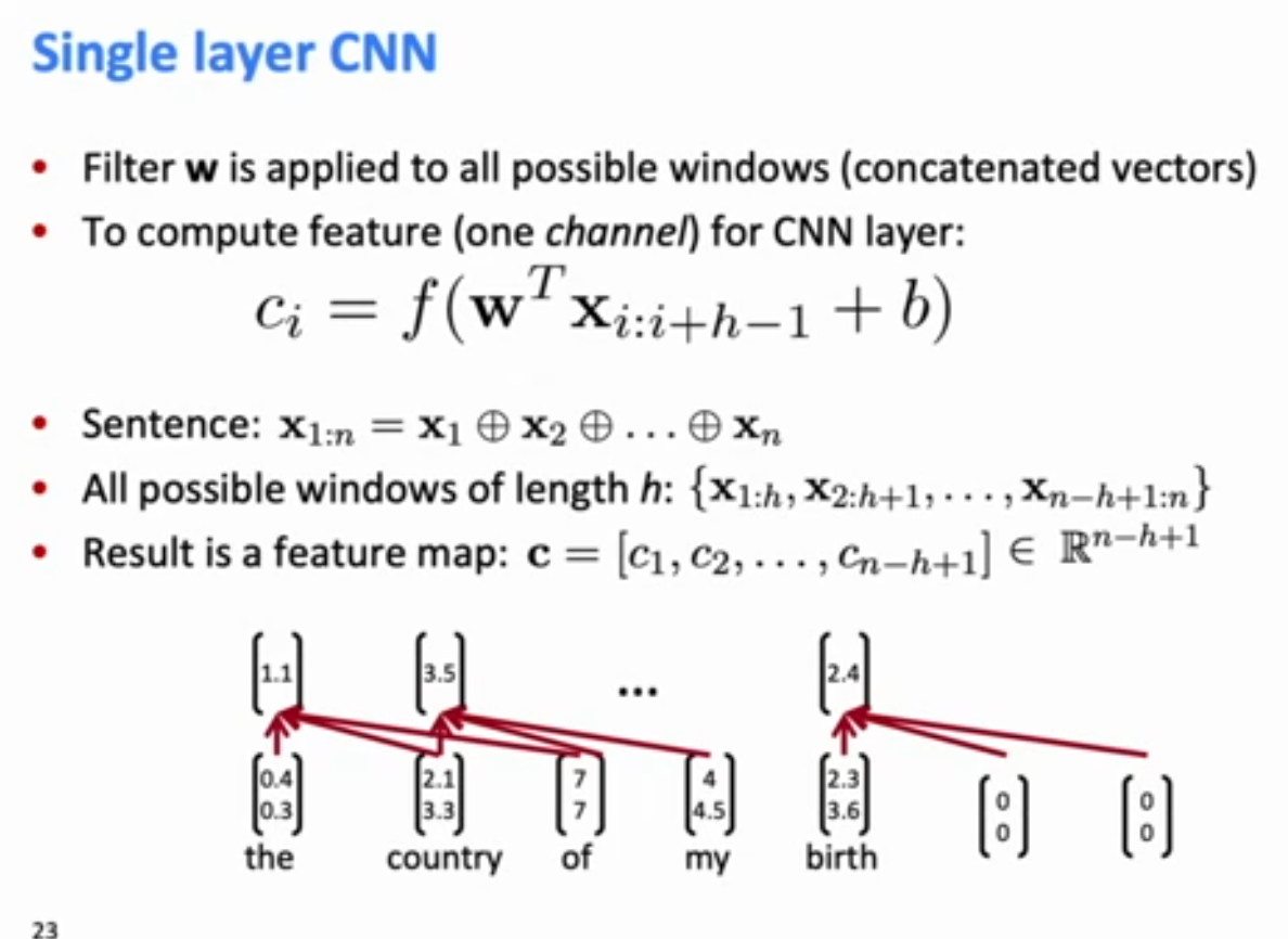
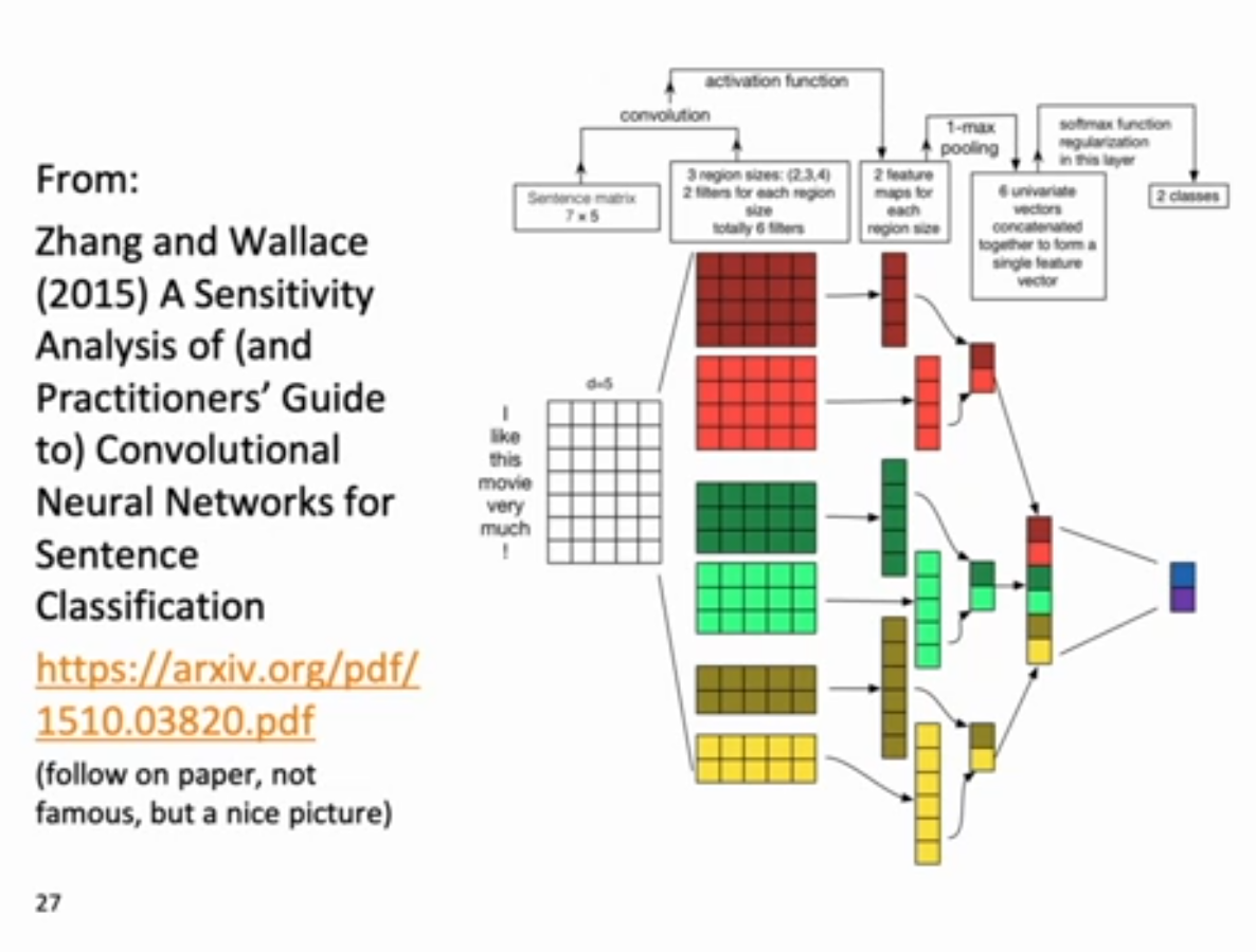
At the end, do maxpooling. They have multiple features of different kernel sizes to do the analysis
He used two identical copies of word vectors (GloVE) concatenated together to represent words. One set was frozen while the other was fine-tuned during training. Elemnts from both copies went in together in the max-pool.
To obtain final feature vector $z = [\hat c_1,…,\hat c_m]$ he used $m=300$, with 100 feature maps each of sizes 3, 4, 5. Finally, the classification was done through a simple softmax layer.
Finally, they used dropout: Create masking vector $r$ of Bernoulli random variables with probability $p$ of being $1$. Delete features during training: $y=softmax(W^{(S)}(r \circ z) + b)$
At test time, no dropout, but becuase before you were dropping out a lot of stuff, scale weight matric by dropout prob $p=0.5$: $\hat W^{(S)} = pW^{(S)}$
Also: Constrain $l_2$ norms of weight vectors of each class to a fixed number s. Not very common. If weights were too large, they were rescaled so that they equal 3. Not very common to do.
Very Deep CNNs for Text Classification (VD-CNN)
(Conneau, Schwenl, LeCun, EACL2017). Starting Point: Build a computer vision-like CNN stack for NLP. This is significant because previous CNNs for NLP has not been very deep.
The authors started from the character level onwards. They truncate or pad documents to 1024 documents.
- For each character, learn a character embedding of dim 16 (dim is not 16x1024)
- Stick that through a convolutional layer with a kernel size of 3 and 64 output channel (dim is now 64x2014)
- For n in 64,128,256,512:
- Stick that through a convolutional block of size (3,n) x2
- Do local pool to halve the size of the size of the sentence but doubple the size of the channels (features). Ourput is size n x 1024/(n/64). Don’t do on last loop.
- Do k-max pooling, keep 8 strongest values in each channel. (Dim=512 x 8)
- Put it through 3 fully connected layers (512x8xnum_classes)
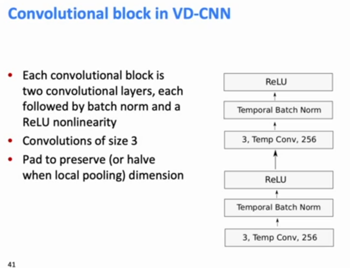
Each Convolutional block is two convolutional layers of kernel 3, each collowed by batch norm and a ReLU nonlinearity. Pad to preserve dimension. Each convolutional block also has a skip connection that goes directly from the start of the block to the end.
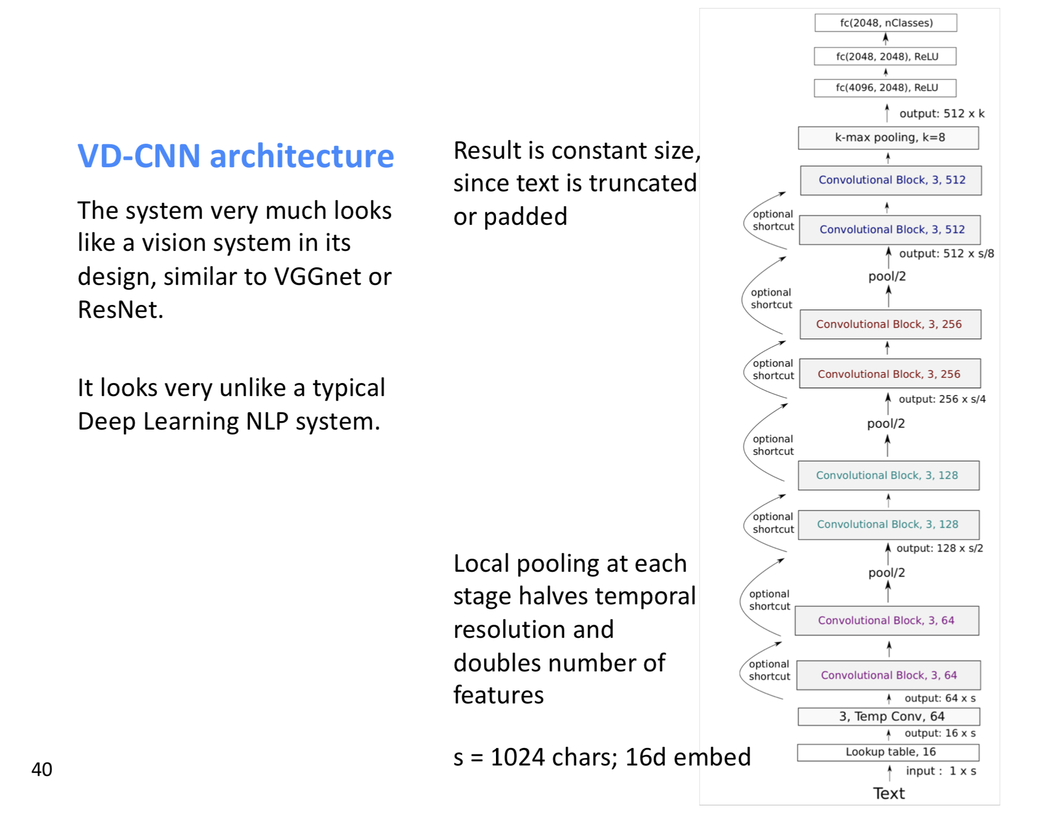
They used huge datasets to test their model Deeper networks work better up to 29 layers, after that point, it didn’t much better with depth.
In vision, people generally use ResNet50 or ReNet101 for good results. They only use ResNet34 for a very lightweigh model. But in language it seems that the model stops improving after depth ~30.
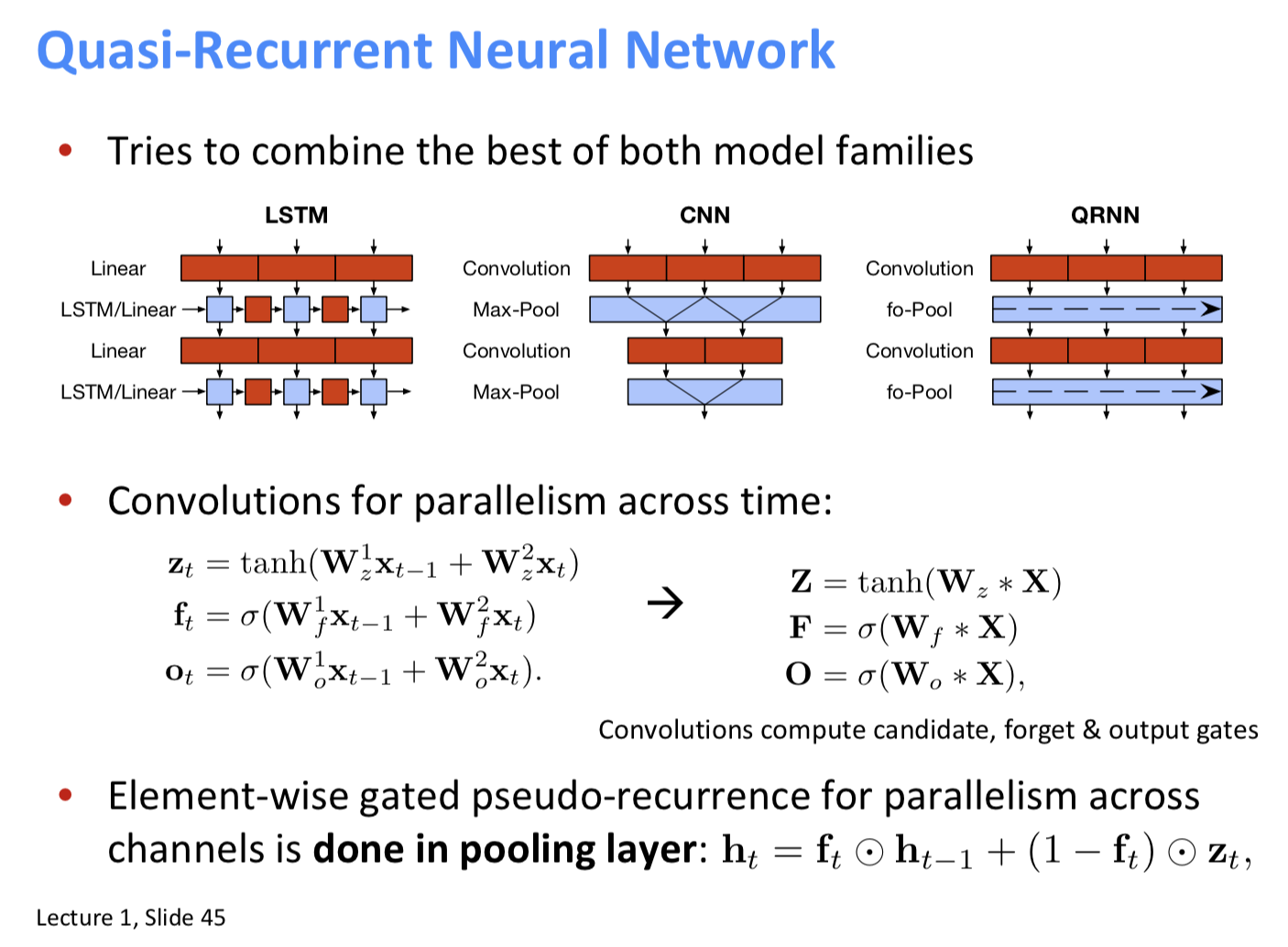
Quasi-Recurrent Neural Networks (Q-RNN, which are actually CNNs)
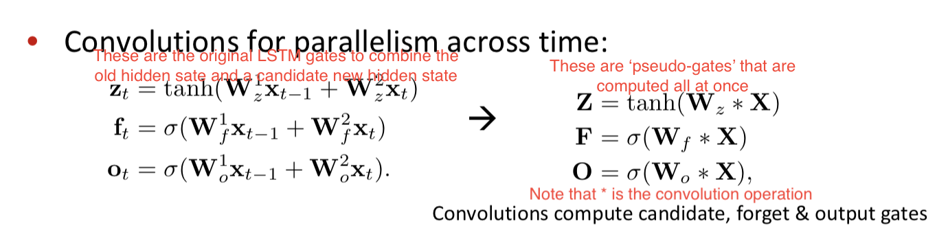
RNNs are a standard building blocks for NLP, but they paralleize badly and slowly. Idea: Take the best and paralleizable parts of RNNs and CNNs.
Rather than doing the standard LSTM things which is calculate the update value and gates for your new time slice, we instaed stick a relation between $t-1$ and $t$ states into the max-pooling layer of a CNN.
So we still compute candidate, forget, and ourput gates, but these candidates and gated values are done inside a pooling layer via a convolutional operation. So element-wise gaten pseudo-recurrence ofr parallelism across channels is done in pooling layer: $h_t = f_t \odot h_{t-1} + (1-f_t) \odot z_t$
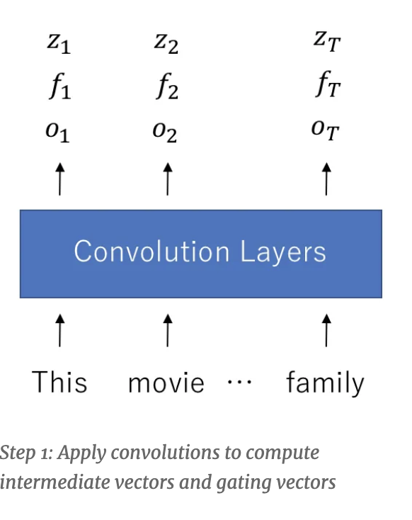
In the pseudo-recurrence, you are modeling an interaction between words and the words next to it at each time slice, but its just worked out locally rather than being carried forward in one layer. But if you made your networks deeper using Q-RNNs, you expand your window of inference and you get a certain window of carry forward interactions.
Q-RNNS are not always better than LSTMs, but they are much faster. Long-term this isn’t the idea that will end up winning out (Transformers will likely be that idea).
More detail about Q-RNNs:
QRNNs use a regular convolution layer in the timestep dimension to compute three vectors for each input: a candidate vector, a forget gate, and an output gate.
More specifically, given an input sequence of $n$-dimensional vectors $x_1, x_2, … x_T$ , the convolution layer for the candidate vectors with $m$ filters produces a sequence of $T$ m-dimensional output vectors $z_1, z_2, …, z_T$. The same goes for the forget gates and output gates. The precise equations are
\begin{align}
z_t = & \tanh(conv_{W_z}(x_t, …, x_{t - k + 1}))
f_t = & \sigma(conv_{W_f}(x_t, …, x_{t - k + 1}))
z_t = & \sigma(conv_{W_o}(x_t, …, x_{t - k + 1}))
\end{align}
This is just a normal convolution. The real magic happens in the pooling layer.
Using the inputs computed above, the QRNN computes the hidden states (outputs) according to the following equation:
\begin{align}
c_t = & f_t \circ c_{t-1} + (1 - f_t) \circ z_t
h_t = & o_t \circ c_t
\end{align}
where $\circ$ is the Hadamard product.
This equation looks like the equation for the LSTM, and the difference may seem a bit unclear at first. The important difference is that the sequential processing only occurs in the pooling layer and that the values of $z_t$, $f_t$, and $o_t$ do not depend on any previous values. This is the essence of QRNNs: do the heavy computation in parallel and do minimal sequential processing in the pooling layers.
That is, the output hidden states of each layer of a Q-RNN at each position do contain some and may be overwritten by some ‘past’ information as determined by the forget and ourput gates, but it can only be as far past as the kernel size.Thus for each layer, the span of dependencies that can be learned in the feature representation is only the kernel size, but longer and longer dependencies can be learned as we increase the depth.
 \
\
General Ideas in ConvNets for NLP
Gating Units used Vertically
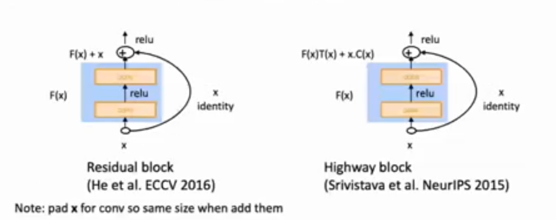
The gating/skipping that we wall in LSTMs and GRUs is a general idea, which is now used in a whole bunch of places. You can also gate vertically between layers of convolutions. Indeed the key idea- summing candidate update with shortcut connection- is needed for very deep networks to work.
##
Residual Block (He et al 2016)
Simple skip connection, used in ResNet. The skipped embedding is added (not concatenated) to the output of the Conv layer.
Highway block (Srivistava et al 2015)
Instead of adding the identity and the Conv layer, multiply the Conv layer outout to a $T$ gate and the identity ourput to a $C$ gate.
The residual block is about just as powerful as a highway block, and it is also simpler. How to interpret the residual block is that the default action is to carry over the identity to the next layer, and the job of the Conv block is to learn the deviations from the identity which should be taken between the layer.
The highway block seems more powerful as you are able to control both how much of the identity and how much of the new signal gets carried forth. But it isn’t really, because you have have the Conv block in the residual network learn the amount of identity signal to lose.
Appendix
(1) 1D CNNs in Pytorch
batch_size = 16
word_embed_size = 4
seq_len = 7
input = torch.randn(batch_size, word_embed_size, seq_len)
conv1 = Conv1d(in_channels=word_embed_size, out_channels=3, kernel_size=3) # can add: padding=1
hidden1 = conv1(input)
hidden2 = torch.max(hidden1, dim=2) # max pool
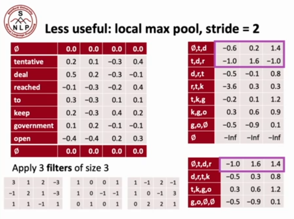
(2) Other less helpful notions: The below are all ways to compress data. They are from vision, not many people actually use them in NLP.
- Stride(2) - We can jump every 2 words in the convolution. Rarely used.
- Local Max Pool, Stride=2. After getting the features from the convolutions, compress the representation into half the size by taking the max of every 2 positions.
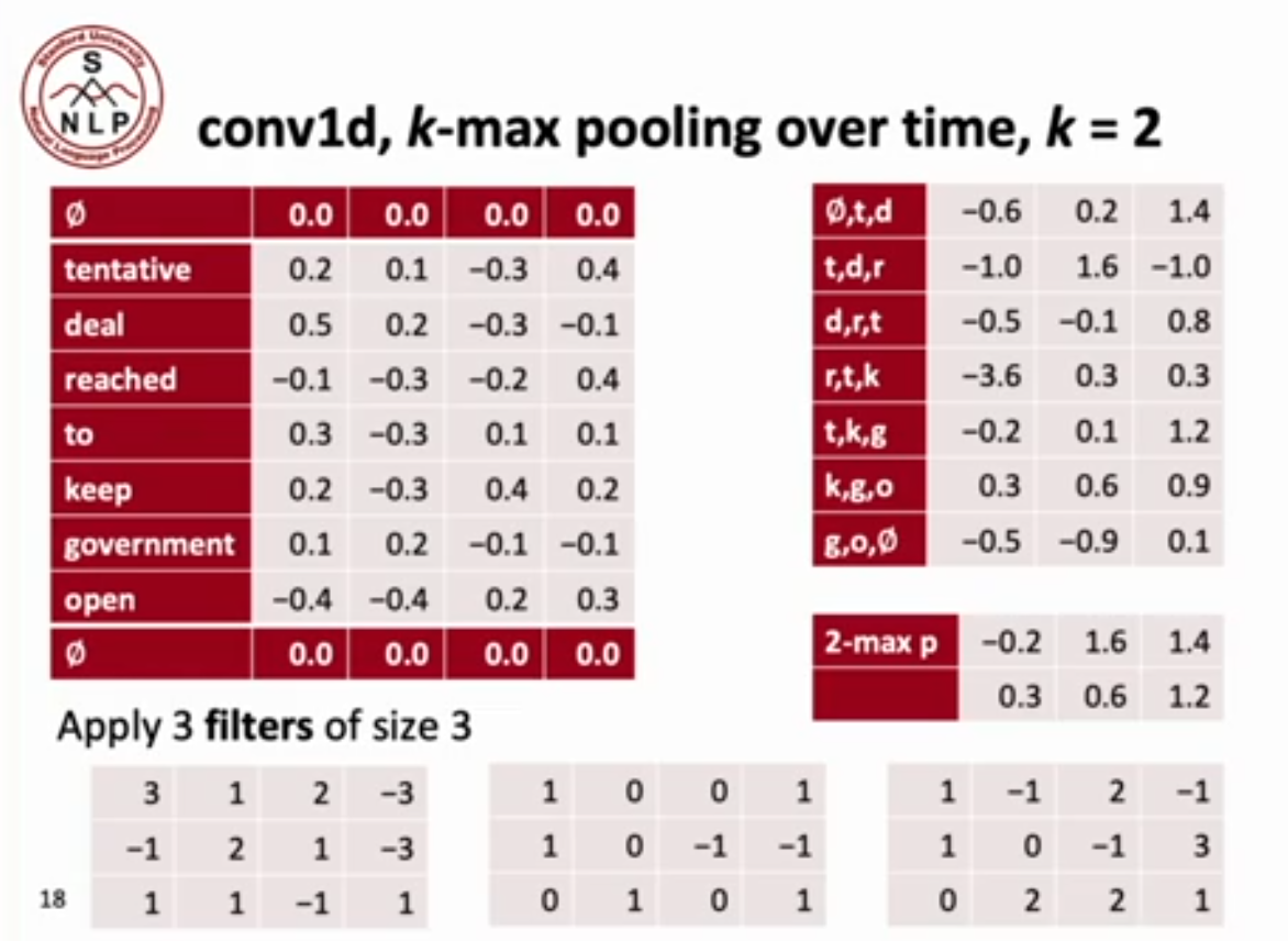
- k-max pooling over time:
- pick the k highest activations in the sequence and keep them in the order they origianlly appeared, throwing out the rest.
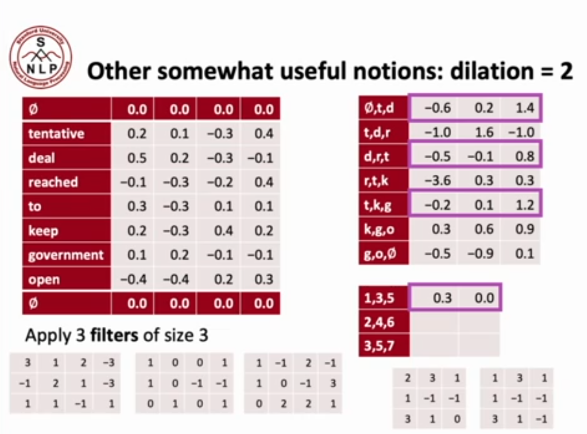
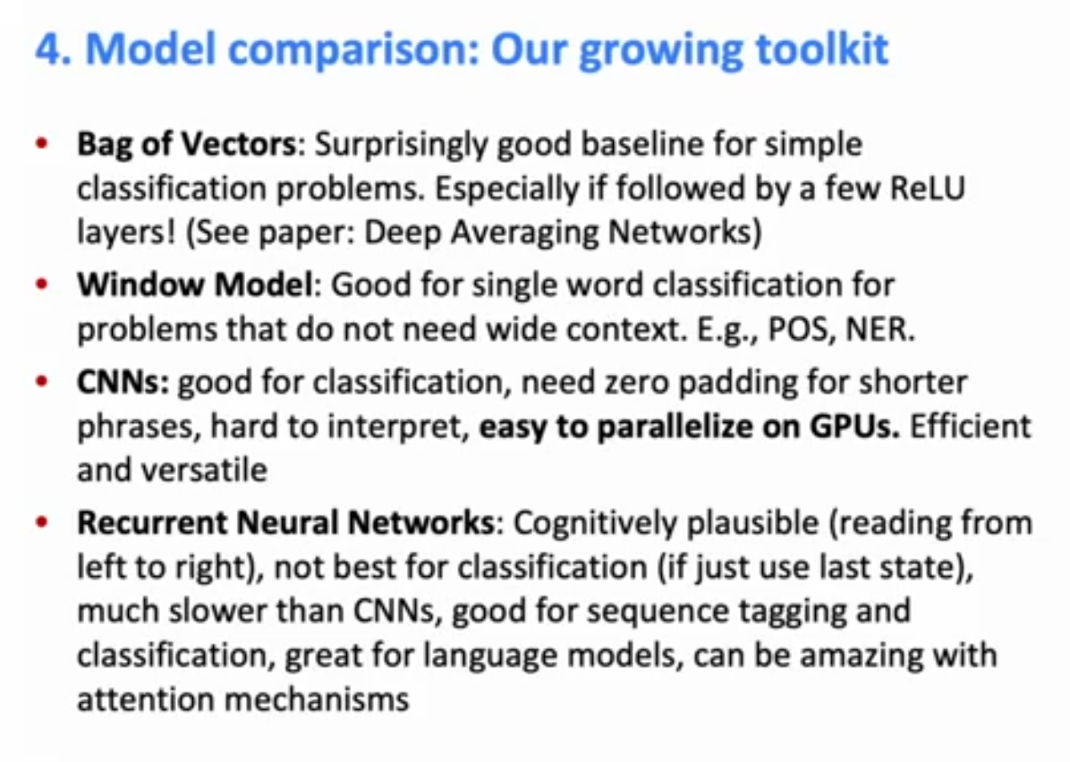
(3) Comparison of models simple to complex:
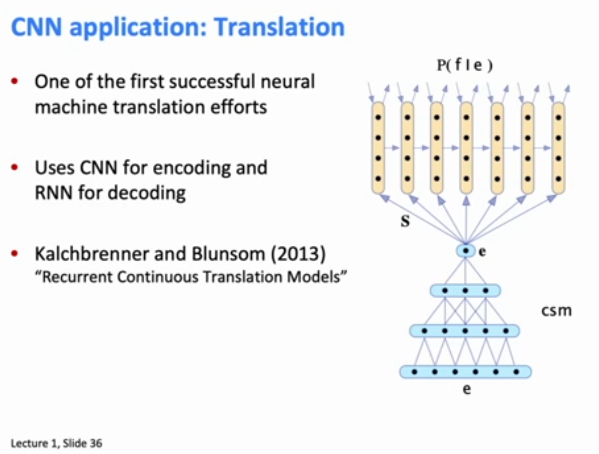
(4) CNN on NMT (2013, very old, the first NMT paper of the modern era)
The encoder was a CNN, which was decoded with a sequence model.
It’s really easy to use CNN as encoders.
It’s harder to use CNNs as decoders (because you have to use masking of future words during training).
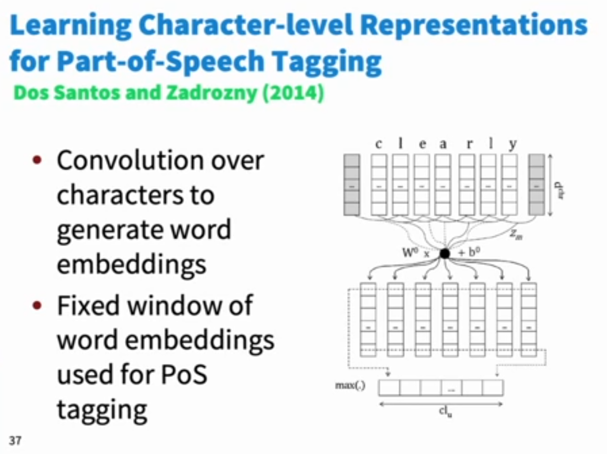
(5) Character level CNNs for POS tagging
Character level CNNs to build a word embedding.