Cs 234 homeworks and midterm
Homework 1
1. Gridworld
1a.
$r_s = 1$ because penalizing actions would cause agents to try take the least number of actions possible to termination. The values for all states then is as follows
| States | Value |
|---|---|
| 12 | 5 |
| 11, 8 | 4 |
| 4,7,10 | 3 |
| 3,6,9 | 2 |
| 2, 13 | 1 |
| 1,14 | 0 |
| 15 | -1 |
| 16 | -2 |
| 5 | -5 |
1b.
States | Value
——-|——
12 | 7
11, 8 | 8
4,7,10 | 9
3,6,9 | 10
2, 13 | 11
1,14 | 12
15 | 13
16 | 14
5 | -3
1c.
\begin{align}
V^\pi_{old} & = \sum_{i=0}^\infty \gamma^i r_i \
V^\pi_{new} & := \sum_{i=0}^\infty \gamma^i (r_i+c)
& = \sum_{i=0}^\infty \gamma^i r_i + \sum_{i=0}^\infty \gamma^i c
& = V^\pi_{old} + c / (1-\gamma)
\end{align}
1d.
Since there is a positive value for taking any action now, the optimal policy would be to keep taking actions and avoid termination. This leads to an infinite value in the unshaded squares.
1e.
Since $\gamma < 1$, the value reached by taking actions and recieving reward 2 for every action ad infinitum will saturate. The saturation value is $2/(1-\gamma)$. Now the optimal policy is to take actions on the unshaded squares until it saturates, and then terminate in square 12. Theoretically it always takes infintely long to saturate, but practically, if $\gamma$ is closer to 0 saturation will come faster, and the difference from taking one more action will be almost perfectly offset by the depreciation of rewards, so termination may happen quicker. (Note: This is somewhat wrong - rewards are discounted from the starting timestep, so an action taken at time 10000 is heavily discounted. So if gamma is small enough, the optimal policy switches to reach the green target square as fast as possible).
1f.
Yes. If $r_s$ is highly negative (say, -1000), then for squares closer to the red square than the green square it is a better policy to move towards the red square and terminate as quickly as possible to avoid the large negative action penalty. The difference in value between the green and red squares (10) won’t be enough to make the red square more desirable as an exit in this case.
2. Values of Different Policies
2.1
Note: Issue with below - I got a negative sign mixed up somewhere but how?
We expand out the right hand side into a telescoping series. The key insight is that
Note that the left hand size of (2.1) is the expected sum of accumulated rewards of following policy $\pi_2$ up till timestep $t$, following policy $\pi_2$ in timestep $t+1$, and then following policy $\pi_1$ thereafter, while the right hand side refers to the expected sum of accumulated rewards of following policy $\pi_2$ up till timestep $t+1$, following policy $\pi_1$ in time step $t+1$ and also thereafter. Thus
\begin{align}
\def\E{\mathbb{E}}
\sum_{t=1}^H \E_{x_t \sim \pi_2} \Big( Q_t^{\pi_1}(x_t,\pi_1(x_t,t)) - Q_t^{\pi_1}(x_t,\pi_2(x_t,t)) \Big) & = \sum_{t=1}^H \E_{x_t \sim \pi_2} Q_t^{\pi_1}(x_t,\pi_1(x_t,t)) - \E_{x_t \sim \pi_2} Q_t^{\pi_1}(x_t,\pi_2(x_t,t))
& = \E_{x_1 \sim \pi_2} Q_1^{\pi_1}(x_1,\pi_1(x_1,1)) - \E_{x_1 \sim \pi_2} Q_1^{\pi_1}(x_1,\pi_2(x_1,1))
& + \E_{x_2 \sim \pi_2} Q_2^{\pi_1}(x_2,\pi_1(x_2,2)) - \E_{x_2 \sim \pi_2} Q_2^{\pi_1}(x_2,\pi_2(x_2,2))
& + \cdots + \E_{x_N \sim \pi_2} Q_N^{\pi_1}(x_N,\pi_1(x_N,N)) - \E_{x_N \sim \pi_2} Q_N^{\pi_1}(x_N,\pi_2(x_N,N))
& = - \E_{x_1 \sim \pi_2} Q_1^{\pi_1}(x_1,\pi_2(x_1,1))
& + \left( \E_{x_1 \sim \pi_2} Q_1^{\pi_1}(x_1,\pi_1(x_1,1)) - \E_{x_2 \sim \pi_2} Q_2^{\pi_1}(x_2,\pi_2(x_2,2)) \right) \
& + \cdots + \left(\E_{x_{N-1} \sim \pi_2} Q_{N-1}^{\pi_1}(x_{N-1},\pi_1(x_{N-1},N-1)) - \E_{x_N \sim \pi_2} Q_N^{\pi_2}(x_N,\pi_2(x_N,N)) \right) \
& + \E_{x_N \sim \pi_2} Q_N^{\pi_1}(x_N,\pi_1(x_N,N))
& = \E_{x_N \sim \pi_2} Q_N^{\pi_1}(x_N,\pi_1(x_N,N)) - \E_{x_1 \sim \pi_2} Q_1^{\pi_1}(x_1,\pi_2(x_1,1))
& = V_1^{\pi_1}(x_1) - V_1^{\pi_2}(x_1)
\end{align}
The last step is because the first term is the expected return following $\pi_2$ for all states, and the the second term is the extepcted return following $\pi_1$ for all states.
3. Fixed Point
3.a
Base case: $n=1$: $|V_2 - V_1|{\infty} = |BV_1 - BV_0|{\infty} \le \gamma^1 |V_1 - V_0|$. Suppose $|V_{n+1} - V_n|\infty\leq \gamma^n |V_1 - V_0|\infty$. Then, $|V_{n+2} - V_{n+1}|{\infty} = |BV{n+1} - BV_n|{\infty} \le \gamma |V{n+1} - V_n|\infty \le \gamma^{n+1} |V_1 - V_0|\infty$, and we are done.
3.b
\begin{align}
|V_{n+c} - V_n|\infty & \leq \sum{i=1}^c |V_{n+i} - V_n|\infty
& \leq \sum{i=1}^\infty |V_{n+i} - V_n|\infty
& \leq \sum{i=1}^\infty \gamma^{n+i} |V_1 - V_0|\infty
& = \left(\sum{i=1}^\infty \gamma^{n+i} \right) |V_1 - V_0|\infty
& = \gamma^n/(1+\gamma) |V_1 - V_0|\infty
\end{align}
3.c
Given any $\epsilon > 0$, we simply take $k > \log_\gamma \left(\frac{\epsilon}{|V_1 - V_0|\infty} \right)$. Then, for any $m,n > k$, $|V_m - V_n |\infty \le |V_{k+1} - V_k |\infty \le \gamma^{k} |V_1 - V_0|\infty \le \epsilon$. Thus, the sequence $V_0, V_1,…$ is Cauchy and thus convergent to some $V$. This implies for large $k$, $| V_{k+1}-V_k |\infty \approx 0 = \implies | BV_k-V_k |\infty \approx 0 \implies BV_k \approx V_k$, so $V_k$ is a fixed point of $B$.
3d.
Suppose the fixed point was not unique, i.e. $\exists V_m, V_n s.t. BV_m = V_m, BV_n = V_n, V_m \ne V_n$. Then, by the Bellman contraction constraint, and $\gamma < 1$,
\begin{align}
|V_m - V_n|\infty = |BV_m - BV_n|\infty
\leq \gamma |V_m - V_n|\infty < |V_m - V_n|\infty
\end{align}
which is a contradiction.
4. Frozen Lake MDP
4d.
Stochasticity increases the number of iterations required to solve the puzzle. The resulting policy is also changed as a result of the transition matrix being different. In the stochastic case, the action chosen is one that has zero probability of leading to a hole (termination without reward) or getting stuck (in an absorbing state with no access to the reward).
Assignment 2
0
0.1
The maximum reward is 4.1. This is obtained by the 3 following trajectories: 002121, 021021, 021210. Note that action 4 is exactly the same as taking the action which lands one in the same state, and thus is superflous. For the other actions, we essentially have two reward regimes: starting out from 2 and not starting out from 2. The reward matrix is below
| finish state | 0 | 1 | 2 | 3 |
|---|---|---|---|---|
| s != 2 | .1 | -.2 | 0 | -.1 |
| s = 2 | -1 | 2 | 0 | 1 |
Note that the minimal reward from not starting out from 2 for all time steps (staying in 0 5 times) is 0.5, lower than the minimum reward if starting from 2. Thus, a policy starting from 2 and picking 1 or 3 once strictly dominates the policy of avoiding starting from 2, and by a parallel argument a policy starting from 2 twice strictly dominates the policy of starting from 2 once. As each start from 2 must first return to 2 before it can start again from 2, it is not possible to start form 2 three times.
Thus, the maximum policy starts from 2 twice, and moreover takes the 2-1 path both times, giving reward 4. The optimal policy thus has form 0(21)(21)*, where one of the three * is replaced with another transition. As it turns out, since in all three cases the start point for * is not 2, the policy value is equivalent no matter which one is picked, and the action which should replace * is the maximizer of the s != 2 case – go to 0. 002121, 021021, 021210 are thus the maximizing trajectories.
1
1.1
The state space may be exceedingly large, instaed of enumerating it explicitly it is much more efficient to use $w$ to function-approximate it.
(Correction:) For each update, we have to find the action which maximizes $\hat q$ at state $s’$. We dont want to compute values over all action separately in separate computations, and then throw away all values except the maximizer. It is more optimal to compute the Q value for any state and any action all at once, from which we can immediately take the max.
1.3
No, this weight update is not an insteace of SGD. The true (stochastic) gradient of equation (3) requires differentiating thorugh not only the $\hat q(s,a ; w)$ term, it also requires differentiating through the $\max_{a’ \in A}\hat q(s’,a’; w)$ term, that is, the true gradient update is
This leads to (4)systematically overestimating the gradient step.
1.4
Yes. If we treat $w^-$ as a constant, then (4) is the accurate stochastic gradient update (scaled by a factor of 0.5) corresponding to the loss in (5). This is because the gradient is only computed with respect to the last term $\hat q(s,a;w)$ and not the term in the middle $\max_{a’ \in A} \hat q(s’,a’;w)$, which we treat as constant.
1.5
If we do not update $w^-$ to $w$ very often ($C$ is very large), then the update factor $r + \gamma \max_{a’ \in A} \hat q(s’,a’;w) - \hat q(s,a;w)$ is wrong and the network will learn the wrong weights. If we update $w^-$ to $w$ too often ($C$ is very small), then each stochastic step will overestimate the true gradient, and, while the network will converge to the true weights in the limit, the learned weights will be biased in the meantime, and training will moreover be unstable.
(Correction:) Less frequent target network updates lead to less informative training targets, but result in Q-network weight update steps more closefly folloing the trye gradient direction. More frequent target network updates causes the gradient direction to be more off by the above analysis.
1.6
The difference betweeh DQN and a pure supervised learning approach is that in pure supervised learning, the data distribution $D$ is known and fixed beforehand, whereas in DQN, the data distribution $D$ (the replay buffer) is generated as the model learns and changes as training goes on.
2
2.1 (?)
Starting from (2), and using the equation that $w^T \delta(s,a) = \hat q(s,a ; w)$, we have
2.2 (?)
Given the definition of $\delta (s,a)$, we have $[\delta(s,a)]^T \delta (s,a)$, so (??? Why is this the same?) (Correction: This is not the same as the solutions but I’m not sure what they really mean)
2.4
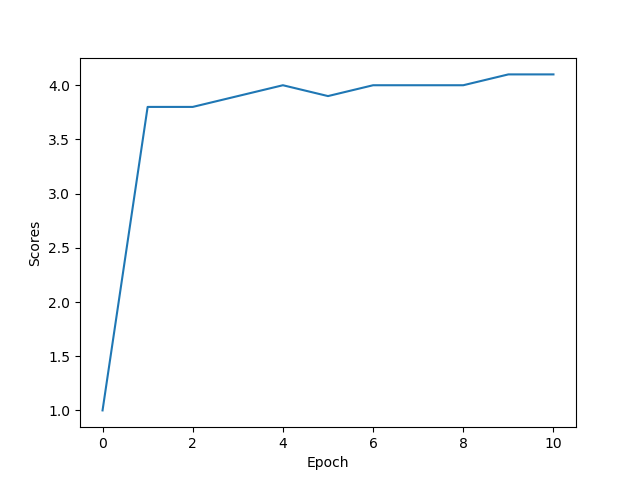
Yes. The score is 4.1.
3
3.2
This model also achieves the highest possible score. The training time took a bit longer to achieve this score. 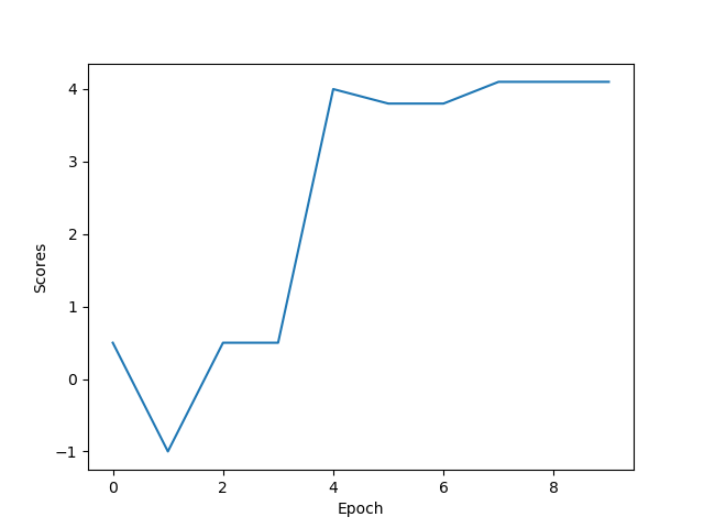
4
5
We know that if we recieve reward sequence $r_t, r_{t+1},\cdots$ following action $a_t$ at time $t$ form $s_t$, then Having taken one step, r_t is certain, and The bias is then Similarly, using the n-step SARSA, the bias is Using the assumption that the current value estimate $\hat q$ is uniformly biased across the state-action space, $\hat q(s_{t+n},a_{t+n}) - \mathbb{E}[r_{t+n} + \gamma r_{t+n+1} + \cdots] = \hat q(s_{t+1},a_{t+1}) - \mathbb{E}[\gamma r_{t+1} + \gamma^2 r_{t+2} + \cdots]$, since from the perspective of the current update the left and right hand sides are just different bias terms starting from different states and taking different actions. We substitute $b$ for this term. Thus, and we are done.
Midterm CS234 Zheng Ma
1
1A
- True
- True
- True
- True
- False
- False ?
- False
1B
- Deterministic $AS^2$. A deterministic policy is determined by $\pi(s,a) = s’$, and there are $AS^2$ different combinations of $(s,a,s’)$. Stochastic: An infinte number, because the distribution of action transitions we can specity are continuous.
- No. The REINFORCE algorithm is a gradient descent algorithm, and only converges to local optima.
- All states are visited an infinite amount of times evnetually
- Inverse RL is a problem in which we train an agent to obtain the policy that matches a teacher’s policy by matching their output steady state distributions. In such a case we wish to pick the policy which matches the teacher’s steady state distrbution but which has the maximum entropy in parameter space as possible. The intuition behind this is that we are worried about overfitting too much to the teacher trajectory. Thus we try to pick the policy which matches the teacher’s state distribution while underfitting as much as possible.
| 1 is $ | A | ^{ | S | }$ in the deterministic case (1pt). 3 is missing the Robbins-Munro conditions (1pt). 4 is vague. (1 pt) |
12/15
2
2a
San Jose
2b
Bus from S1 and S2, Train from S3
2c
Yes. The optimal policy is bus from S12, train from S3 to S12. The rewards are no longer Markovian, but that is not important for our case. We only care that the true optimal policy can be expressed in terms of the new representation.
2d
Because Q learning bootstraps, it makes use of the Markov Assumption, that the expected reward from state S12 is independent of how S12 was reached. This is not the case in reality; the expected reward is in reality higher when S12 was reached by train rather than by bus. Thus, Q-learning estimates the entire future reward trajectory with a single estimate for $Q(S12, a), a\in (Bus, Train)$, regardless of how S12 was reached. Given this, and ignoring the fact that the action we take from S3 affects future rewards from S12 using the Markov assumption, the best single-step action to take from S3 is to bus, which produces higher rewards. The optimal action is to train only because higher rewards will accrue to that action only two timesteps ahead, but using the Markov assumption we only explicitly look forward one time-step.
2e
Technically, the Monte Carlo Policy evaluation would never terminate in the non-episodic case, but we can set it to terminate at a high time-step or when policy values start converging.
THe Monte Carlo Policy evaluation would find the same policy as (c), as it evaluates all actions in conjunction with other actions until the end of the episode in order to compute the policy value. It would determine that the value of using the combination of train from S3 -> S12, bus from S12 -> S3 produces a higher value than any other the other policies.
14/14
3
3a
| s | a | r | s’ |
|---|---|---|---|
| s1 | a1 | 3 | s2 |
| s1 | a2 | -1 | s2 |
| s2 | a1 | -2 | s1 |
| s2 | a2 | -1 | s2 |
We cannot have $\gamma = 1$ because then the value is unbounded, henece we assume $\gamma < 1$. In this particular case, we assume $\gamma > 2/3$. In the above MDP, the true best policy is (s2,a1),(s1,a1).
The value of state s1 is $3-2\gamma +3\gamma^2 -2\gamma^3 + \cdots = \frac{3-2\gamma}{1-\gamma^2} > 0$. The value of state s2 is $-2 +3\gamma -2\gamma^2 + 3\gamma^3 + \cdots = \frac{-2+3\gamma}{1-\gamma^2} > 0$ since we assumed $\gamma > 2/3$.
Starting from $V(s1)=V(s2)=0$, the first value iteration update for the value is
Thus, $V(s2)$ moved from 0 to negative, further away from the true value of $\frac{-2+3\gamma}{1-\gamma^2} > 0$.
3b
The contraction property of the Bellman Backup operator states that the infinity norm (max over states) of the value function over states must not increase after every application of the Bellman Backup. However, this is not at all in consistent with a situation where the max divergence from the optimum decreases, but the divergence of some other state which does not produce the maximum divergence increases.
10/10
4
4A
4Aa
where $G_{it}$ is the sum of all future rewards obtained by following the policy and reciving transitions and rewards according to the lookup table.
4Ab
No bootstrapping. The $G_{it}$ term is a sample, since the update is only performed with respect to one particular (sampled) trajectory, and this sampling is done to estimate the actual optimal Q value which is obtained in expectation over trajectories.
4Ac
Assuming we have $G_{it}$ cached for each $t$, the computation complexity to perform the MC update is $O(t)$ where $t$ is the number of time-steps in the episode.
THe MC update goes through the episode and either incrementally or at the first visit to each state, updates the Q value for that state and the particular action taken at that timestep according to the update equation above. Since $G_{it}$ and $Q^\pi(s,a)$ can be obtained by a table lookup, the update is constant time, thus to full update is $O(t)$ linear time. (early stopping may be introduced in the first-visit case if each state is visited once early on)
If $G_{it}$ must be computed on the fly, it can be done once for all in linear time simply by caching accumulated rewards from the end to the beginning, and then using those cached accumualted rewards in the linear-time Q updates. The time complexity is thus still linear in $t$.
4B
4Ba
The TD learning update is $max_{a’} Q(s’,a’)$ involves sampling: only one action is sampled (in the Q learning case, always the greedy best single action given the current Q values). $r + \gamma max_{a’} Q(s’,a’)$ involves bootstrapping. We bootstrap our learning with a target which is $r + \gamma max_{a’} Q(s’,a’)$. Q-learning moves the Q function iteratively closer to this value of our recieved target.
Correction: This is Q-learning. Drop the max. Oops. 11/15
5
5A
Depends. In this case the Q function has converged. If the linear value function is roubst enough to parameterize the optimal policy, then the Q function has converged to the value of that optimal policy, and the answer is ‘yes’. However, the linear value function approximation may not be roubst enough to parameterize the optimal policy, in which case we have not discovered the optimal policy, only the best policy that the parameterization can find, and the answer is ‘no’.
Correction. Answer is No. Q value may change with iterations and hence the extracted greedy policy will not in general be optimal, it can still chagne. Or we may have converged to a local minimum.
5B
I would pick S100. S2 does not have enough representational capacity to compute a difficult boundary (with only 2 hidden nodes, a lot of information is lost on the way to the output layer). D10 is probably too deep for our use case, and since we are using sigmoid activations, gradient saturation will make this network near impossible to train. S100 has sufficient representational capacity and is also trainable, despite having much more trainable parameters than the other two (see below).
S2: 2 + 1 ~~ 3 S100: 10x100 + 100 x1 ~~ 10^3 D10: 10x10x10 ~~ 10^3
Correction: Should be D10, for higher representational capacity. 3/8
6
6A
$Q^_1(s_1,\pi^(s_1,1)) - Q^*_1(s_1,a)$
6B
Done in the Homework (Assignment 2)
6C
\begin{align}
$V_1^(s_1) - V_1^\pi(s_1) & = \sum_{t=1}^H (Q_t^(s_t, \pi^(s_t,t)) - Q_t^(s_t,\pi(s_t,t)))
& \le \sum_{t=1}^H (\tilde Q_t(s_t, \pi^*(s_t,t)) - \tilde Q_t(s_t,\pi(s_t,t))) + 2 \epsilon H
\end{align}
… how to continue?
See solutions. Partial credit
11/15
Total score: 12 14 10 11 3 11 = 61/72 = 85%