Cs 224n lecture 6,7 rnn, lstm, gru, language models
Langauge Model - a system that assigns a probability to a piece of text
N-gram langauge models - The last word only depends on the last n-1 words with probability proportional to the probability that the last word followed in the corpus given the last n-1 words. Back off to a n-1 gram language model if the previous n-1 words never appeared.
- You also need to store a huge number of n-grams to do a good n-gram language model.
Basic Neural Langauge Model (Naive)-
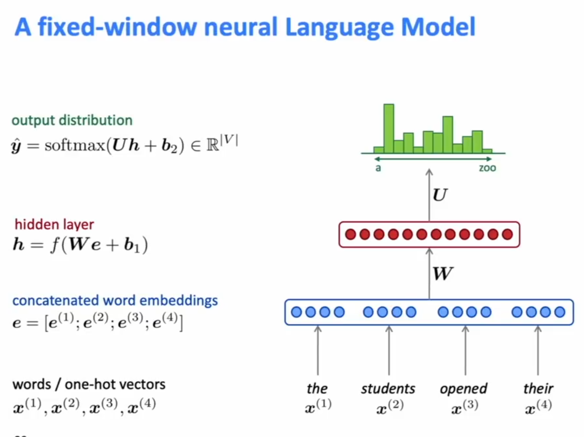
Fixed window neural model - throw away the whole sentence except for the context (like prev 4 words), concatenate teh word embeddings for those 4 words, put it through a hidden layer and a softmax. The issue here is that the fixed window is too small.
RNN Language Models
** **
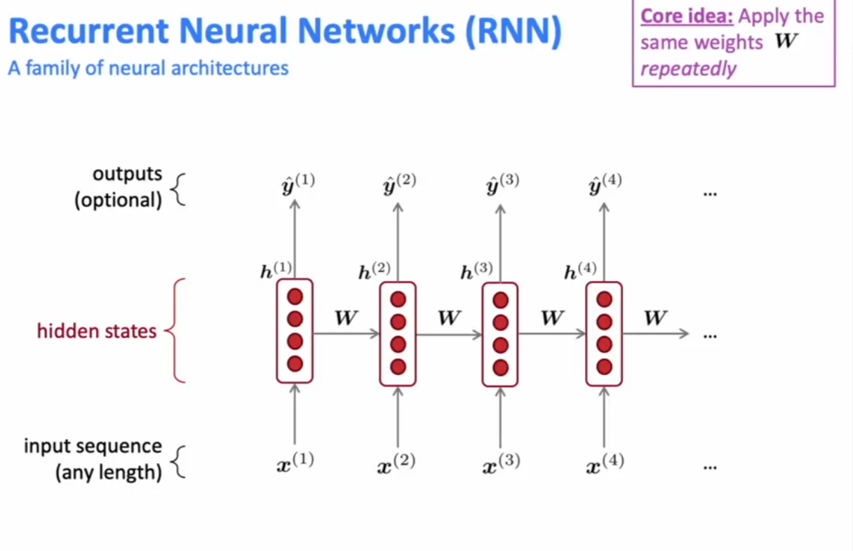
**Core idea of RNNs: **The same weight matrix is applied at every time step of the RNN.
RNN model size doesn’t increase for longer input.
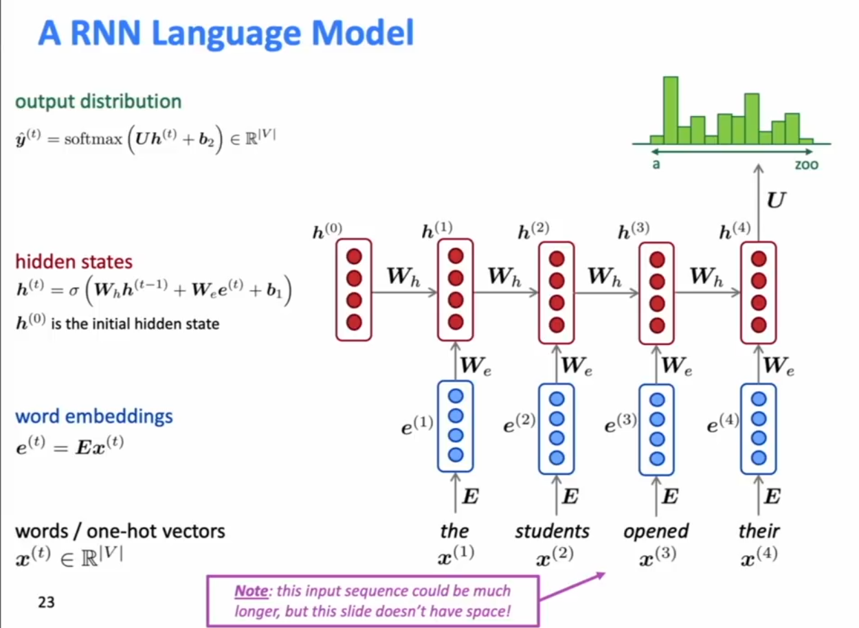
Note that when computing the hidden states, $\sigma$ is any non-linearity and is usually ReLU, not the sigmoid function.
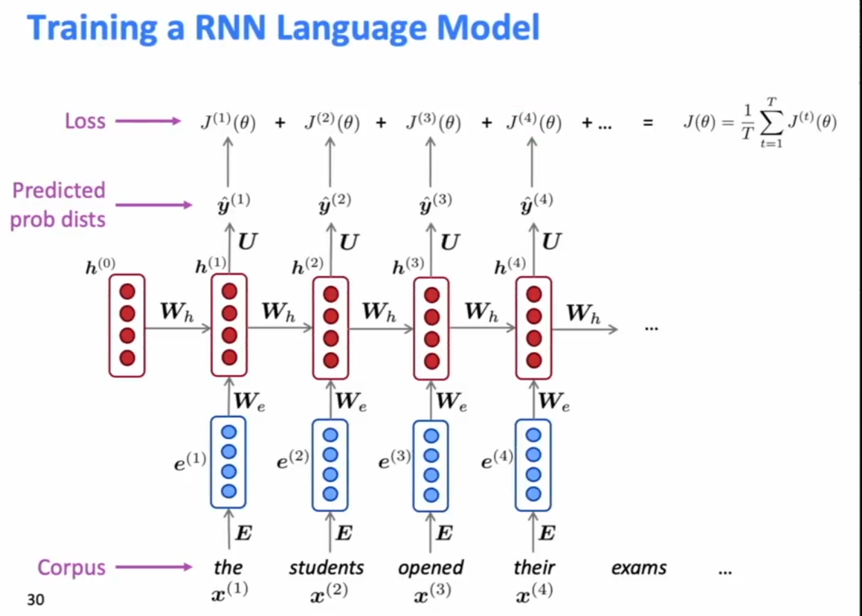
Training a RNN Langauge Model
Get a big corpus of text, feed into the RNN-LM, and compute the output distribution $\hat y ^{(t)}$ for every time step $t$. i.e. predict probability dist of every word, given words so far. The loss function on step t is the CE loss between predicted probability distribution $\hat y ^{(t)}$ and the next true word $y^{(t)}$ (one-hot for $x^{(t+1)}$): Average this to get overall loss for entire training set
In practice, computing the loss and gradients across entire corpus is too expensive, and we consider the sequence of words to use as a sentence or a document instead. We compute loss $J(\theta)$ for a batch of sentences, compute gradients, and update weights, and repeat as in minibatch SGD.
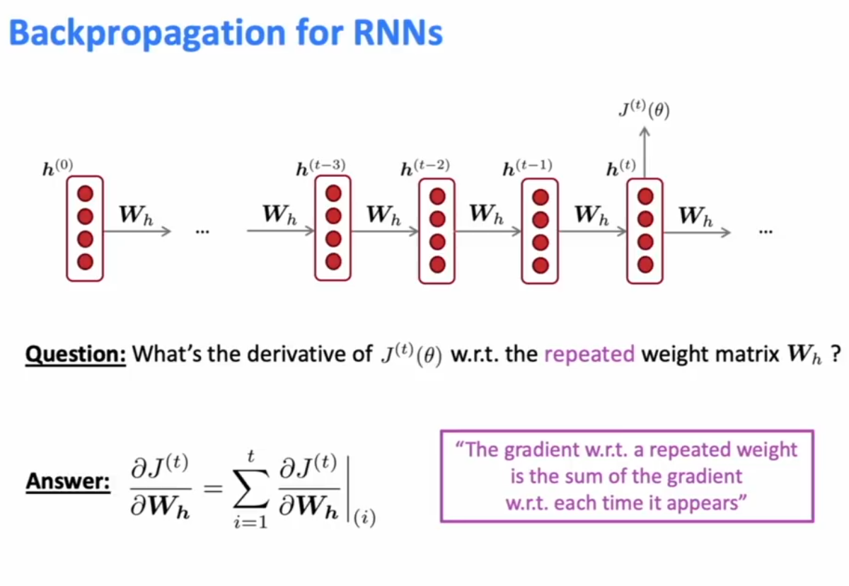
Backpropagation for RNNs:
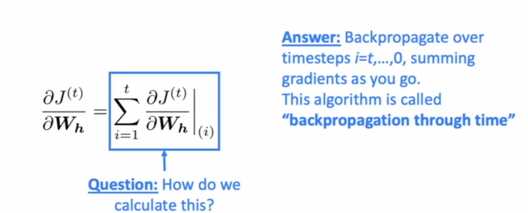
Use backpropagation through time- “The gradient w.r.t a repeated weight is the sum of the gradient w.r.t each time it appears”. In other words, Back-propagate the error, e, back across the whole unfolded network. Sum the weight changes in the k instances of W together.
You can also do character level language models, language models that are conditioned on a certain input.
Evaluating Langauge Models - Perplexity (the Prob of the Corpus)
**The standard evaluation metric for Language Models is Perplexity = **the inverse probability of the corpus, given the language model, normalized by the number of words. Lower perplexity is better!
Perplexity is equal to the exponential of the cross-entropy loss $J(\theta)$.
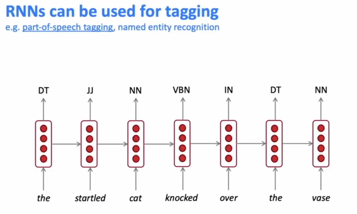
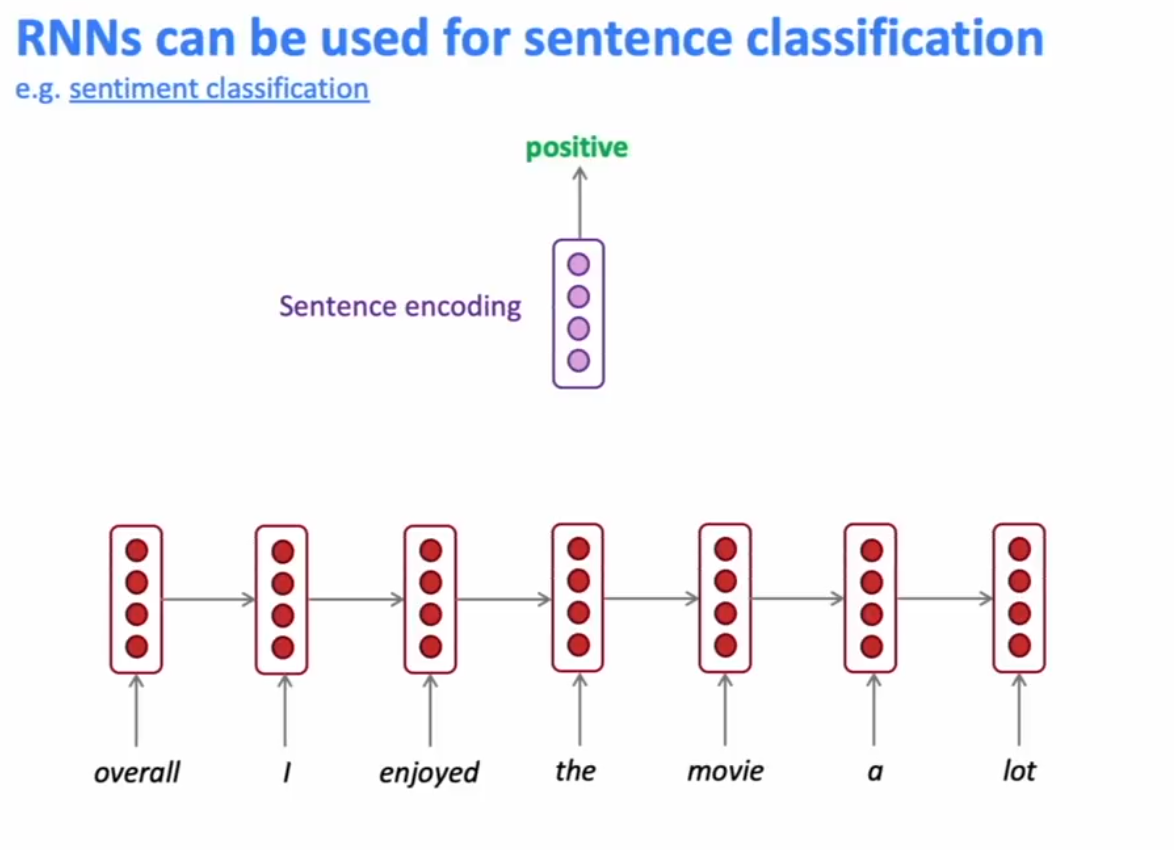
Other Uses of RNNs RNNs can also be used for part-of-speech tagging and named entity recognition. RNNs can be used for sentence classification (ie. sentiment classification).
- Basic way - use the final hidden state as the sentence encoding
- Usually Better Way - use the element-wise max or mean of all hidden states as the sentence encoding.
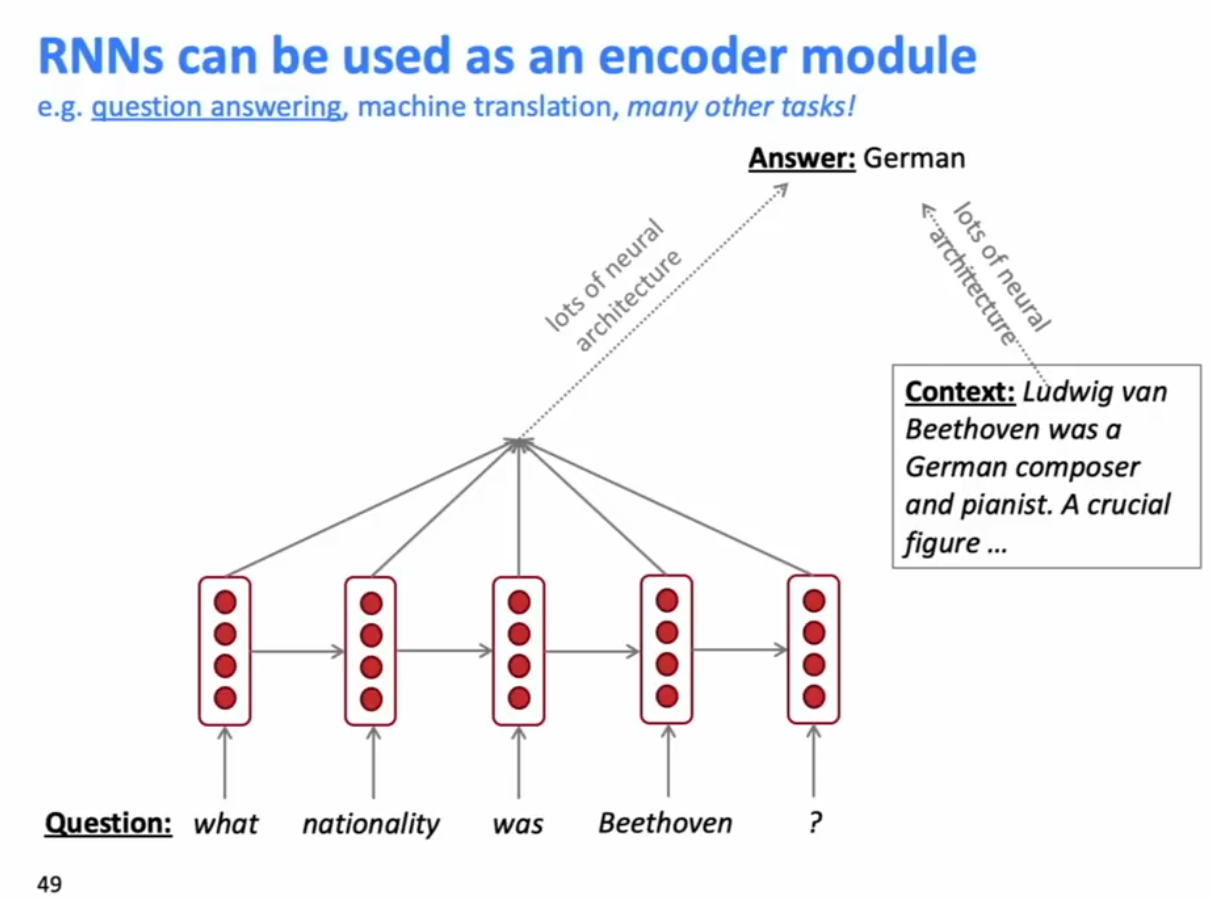
RNN can be used as an encoder module, by taking the hidden states as the encoded state.
- ie for Question Answering
- For Machine Translationn
RNN-LMs can be used to generate text, through a conditional language model.
- Speech recognition, machine translation, summarization.
RNNs can also be used for time-series analysis.
Exploding Gradients
Exploding gradients make all of your parameters +Inf or NaN. Solution-
Gradient Clipping: If the norm of the gradient is greater than some threshold, scale it down to some threshold before applying SGD update. I.e. Take a step in the same direction, but a smaller step. If $||\hat g|| \ge$ threshold:
-
$\hat g \leftarrow \frac{threshold}{ \hat g } \hat g$
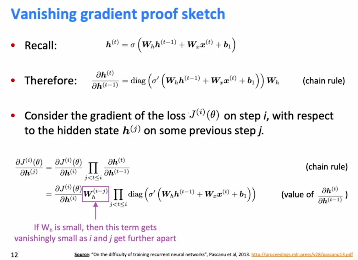
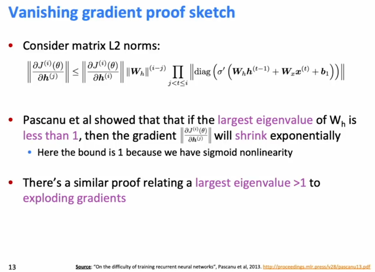
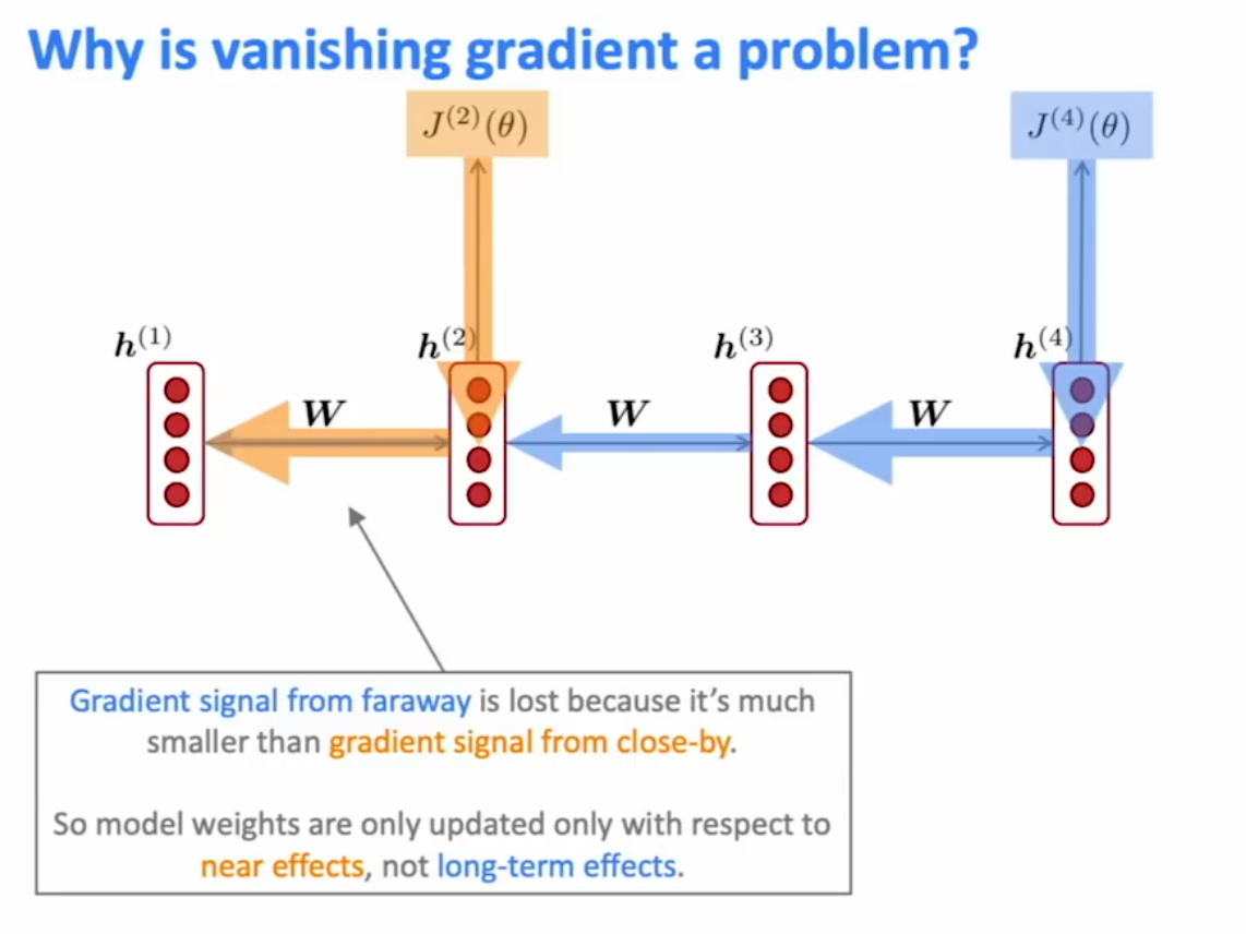
Vanishing Gradients
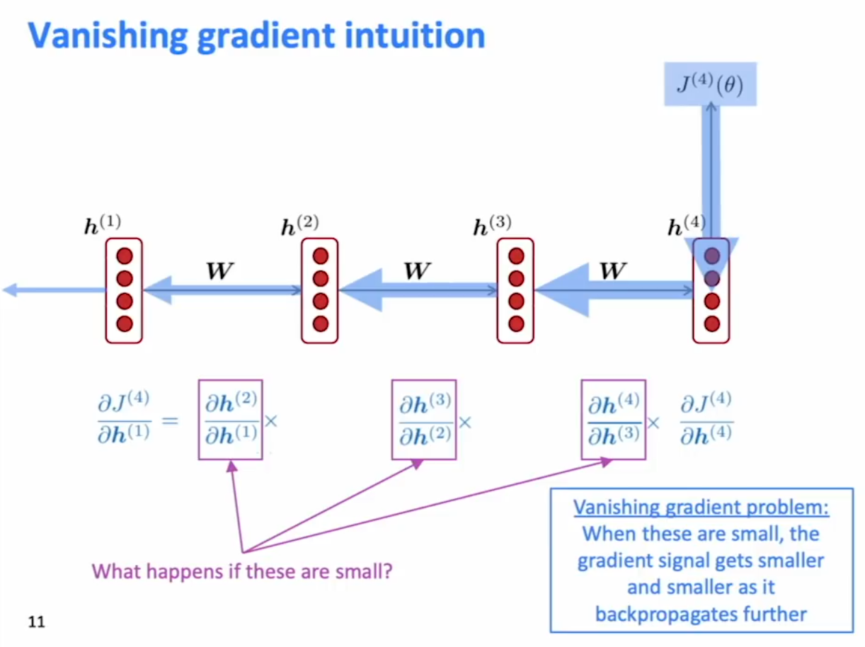
See Appendix 1 for Vanishing Gradient Proof Sketch.
 **
**
**
**
So if there is no signal from timestep t * to timestep *t+n, we can’t tell whether there is really no dependency between step t and t+n in the data or if we have the wrong parameters that lose gradient to capture a true dependency that is in fact there.
LSTM
LSTMs are RNNs with both a hidden state $h^(t)$ and a cell state $c^{(t)}$. Both are vectors of length $n$, and the cell stores long-term information. The LSTN can erase, write, and read information from the cell.
The selection of which information is created/written/read is controlled by three corresponding gates.
- The gates are also vectors of length $n$.
- On each timestep, each element of the gates can be open (1), closed (0), or somewhere in-between. The gates ar edynamic: their value is computed based on the current context.
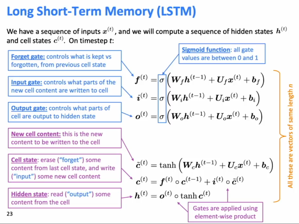
Note that the last tanh is just a nonlinearity.
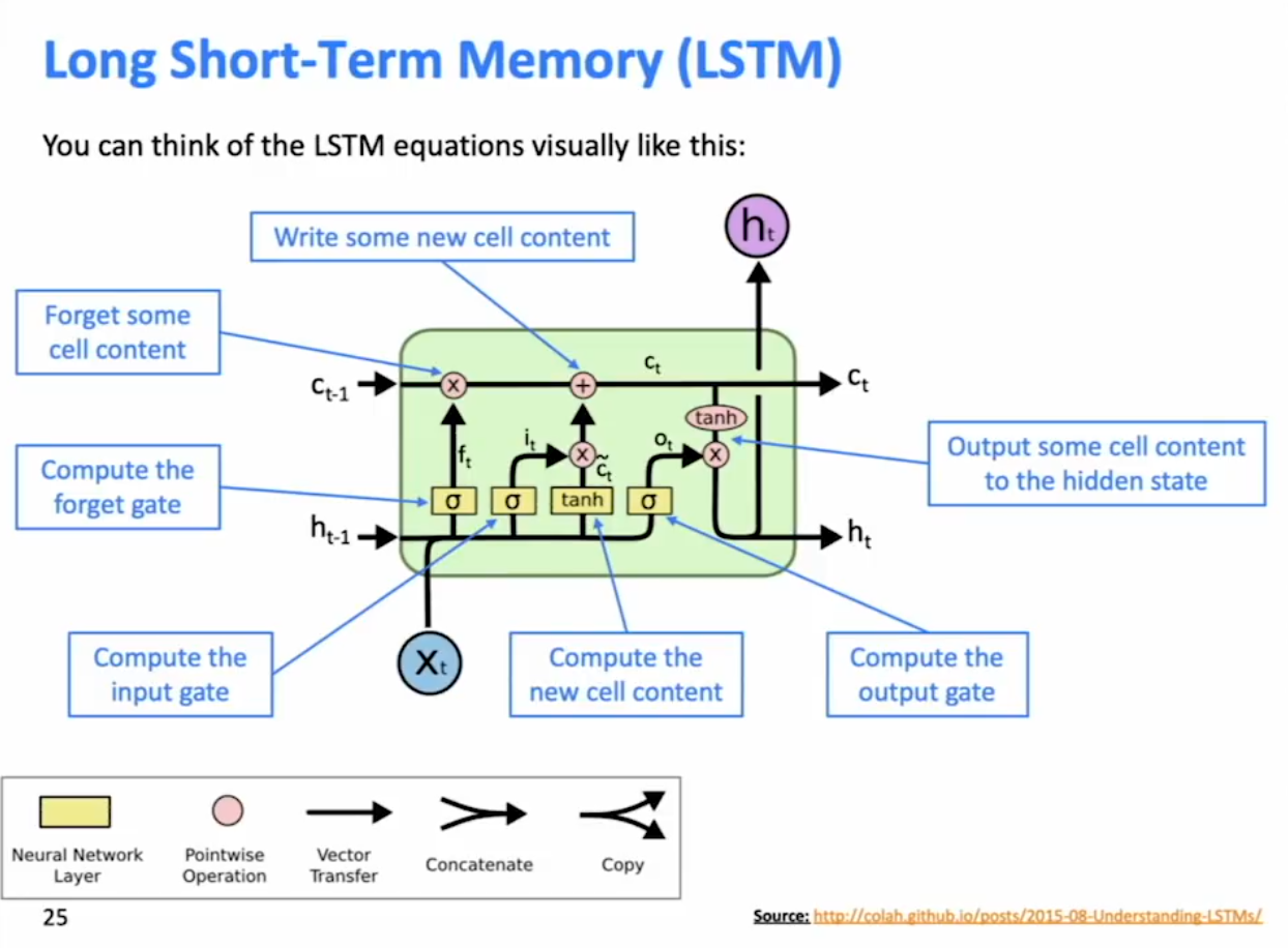
LSTMs inernals are are hard and even the TA doesn’t know the answer to all the problems. (Appendix 2)
LSTM makes it easlier for the RNN to preserve information over many time steps - if the forget gate is set to remember everything on every timestep, then the info in the cell is preserved indefinitely.
LSTM were SOTA in 2013-2015 in NLP. They are still SOTA in some applications but gradually replaced by Transforme
GRU
GGRU does not have the cell states, and only has the hidden states. But they still use two gates: update gate (playing the role of both input and forget gate of LSTM) and reset gate.
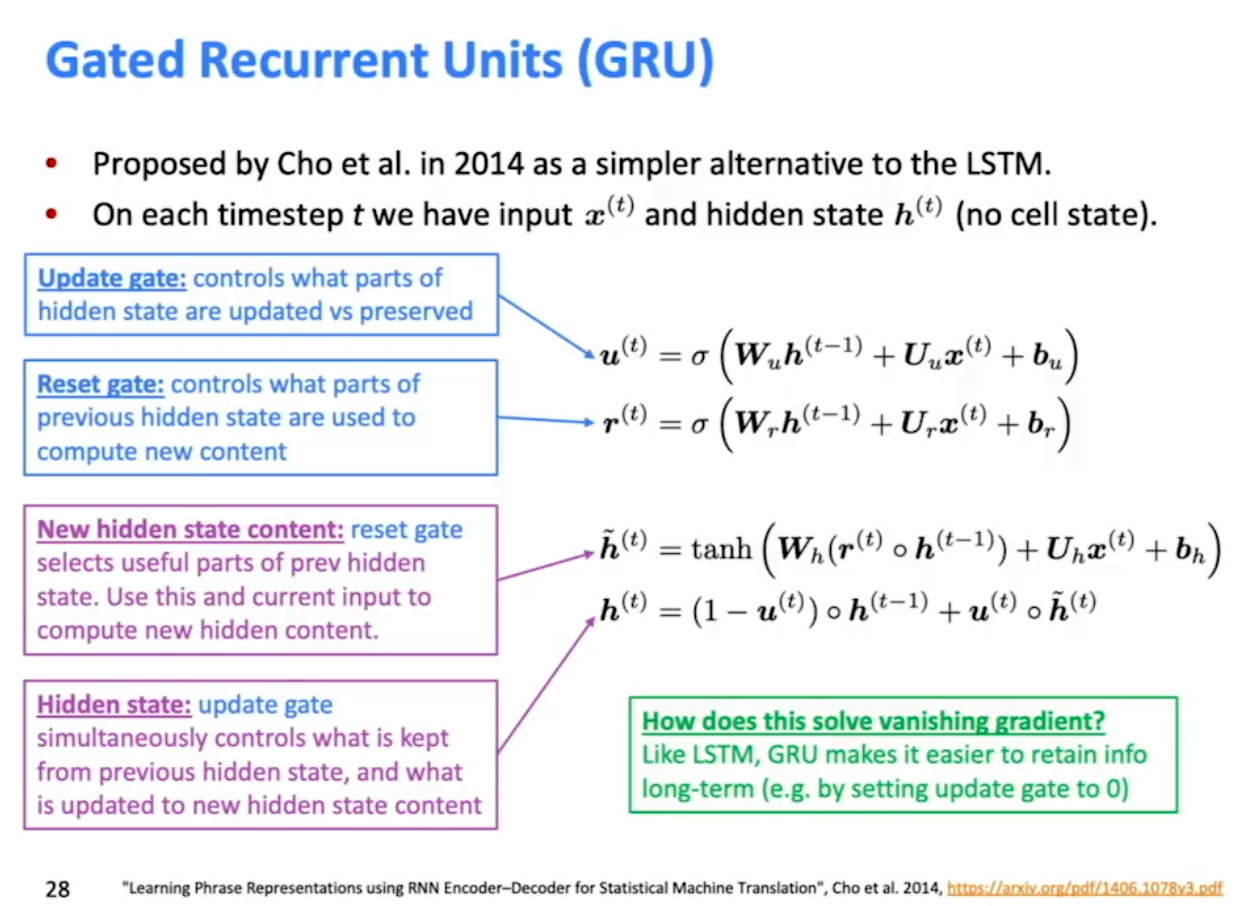
LSTM vs GRU
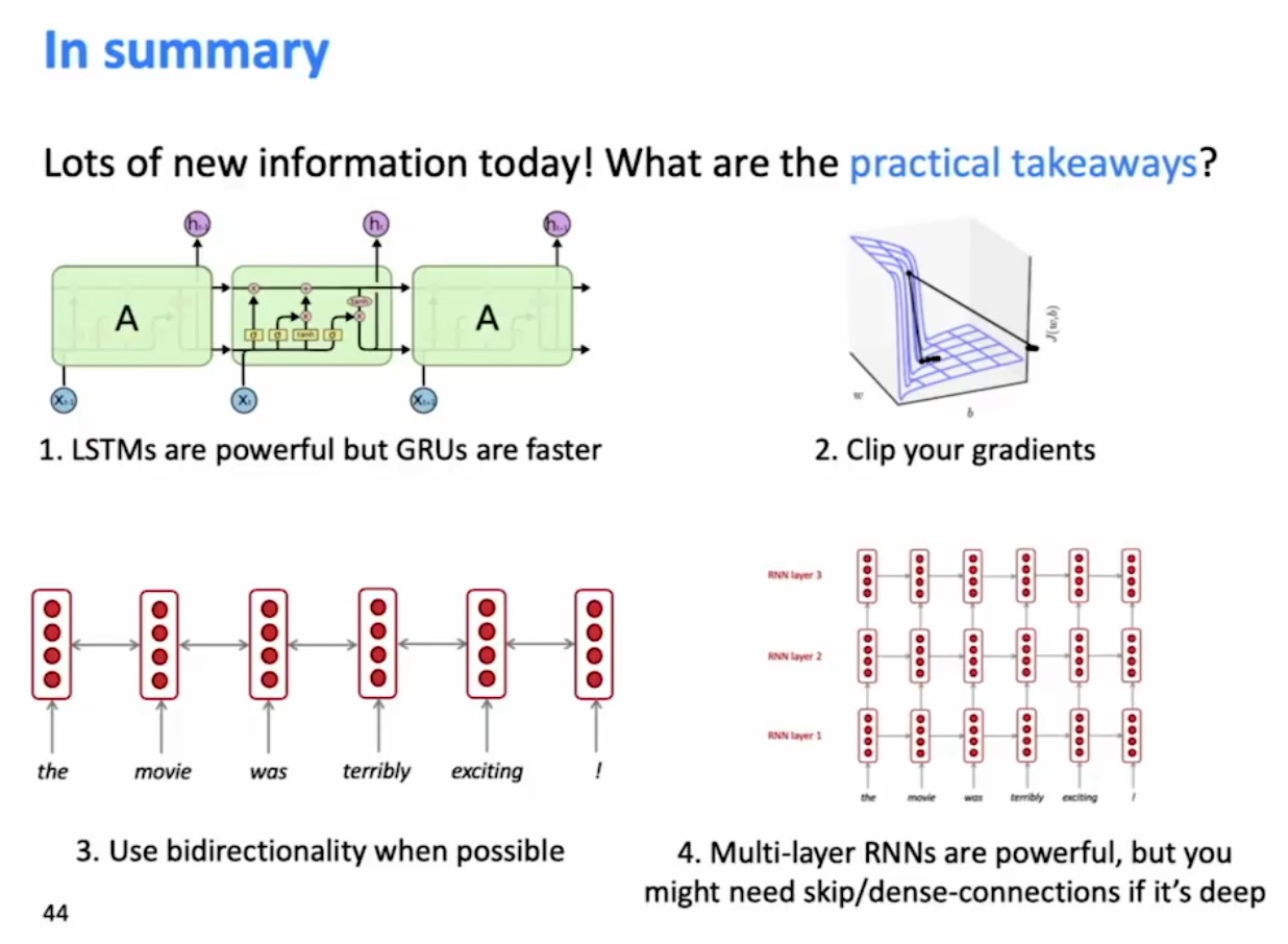
The biggest difference is GRU is quicker to compute and has fewer parameters, but they have similar performance. LSTM is a good default choice, but switch to GRU if you want something more efficient.
Bidirectional RNNs
Ordinary RNNs only capture encodings of the left context in the hidden state. In general it is useful to have both the left and right context. We achieve this by running two completely separate RNNs with different W matrices, one forward through the text and one backwards through the text, and concatenating their hidden states.
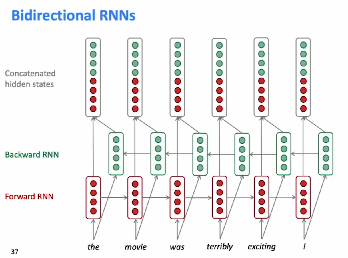
Note: You can’t use bidiectional RNNs when you don’t have reverse context, e.g. language modeling. You should use bi-directional RNNs whenever you can.
ie. BERT (Bidirectional Encoder Representaitons from Transformers) is an example of a powerful pretrained contextual representaiton system built on bidirectionally.
Multi-Layer RNNs aka stacked RNNs
The hidden states from one RNN layer are used as the inputs to the next RNN layer. The lower RNNs should compute lower level features (i.e. syntax) and the higher RNNs should compute higher-level features (i.e. semantics).
If the RNN layers are bidirectional, you would have to compute all of layer 1 before computing layer 2, but if the RNN layers are uni-directional, you can compute the deep layers and the time-steps at the same time (triangular computation, both move up and move right). Thus computing unidirectional multiple layer stacked RNNs shouldn’t take much longer than a unidirectional single layer RNN.
In general, if you are able, use bi-directional Multi-layer RNNs.
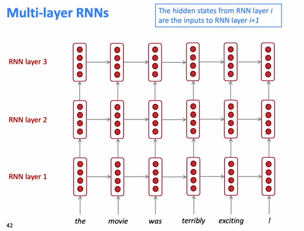
High performing RNNs are often 2 -4 layer multi-layer RNNs or 8 layer RNNs if we add skip connections. It’s hard to learn post 4 layers without skip connections. It’s also hard to get really deep RNNs is because RNNs have to be trained sequentially so training speed gets slower with each layer.
Is vanishing/exploding gradient just an RNN problem
Nope - Though RNNs tend to be more unstable because you are multiplying by the same weight matrix over and over, vanishing/exploding gradients is a problem for any deep network! Solutions:
-** Residual Connections**/ Skip Connection (ResNet, He et al). Note that the skip connection is added (elementwise) to the output of the weight layer, and not concatenated!
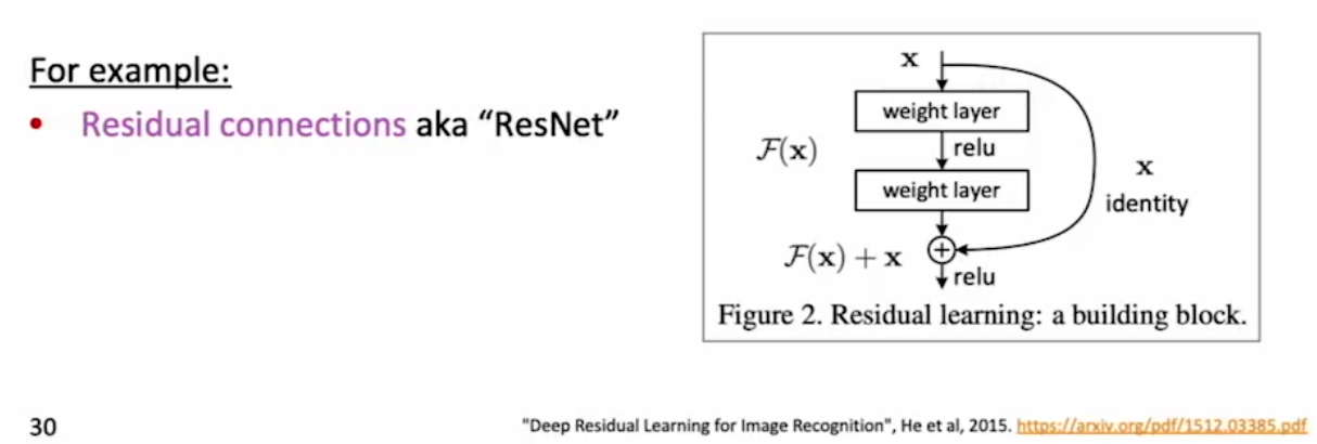
Why add and when to sometimes concatenate - form StackOverflow (the difference is less than one might think!) - Adding is nice if you want to interpret one of the inputs as a residual “correction” or “delta” to the other input. For example, the residual connections in ResNet are often interpreted as successively refining the feature maps. Concatenating may be more natural if the two inputs aren’t very closely related. However, the difference is smaller than you may think. Link
-
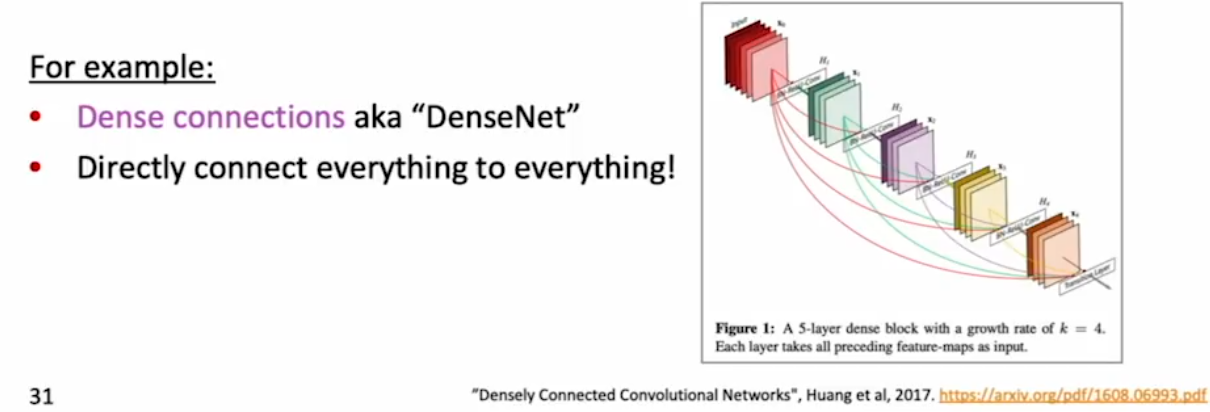
**Dense Connections **(DenseNet) - Add skip connections from all layers to all layers!
-
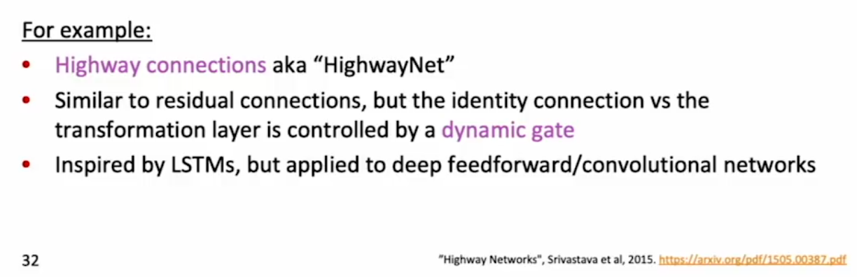
Highway Connections (HighwayNet) - Similar to residual connections but the identity connection vs the transformation layer is controlled by a dynamic gate. Inspired by LSTMs, Highway connections are applied to deep feedforward/convolutional networks.
 **
**
**
**
** **
My own notes on the LSTM GRUs, RNNs in general:
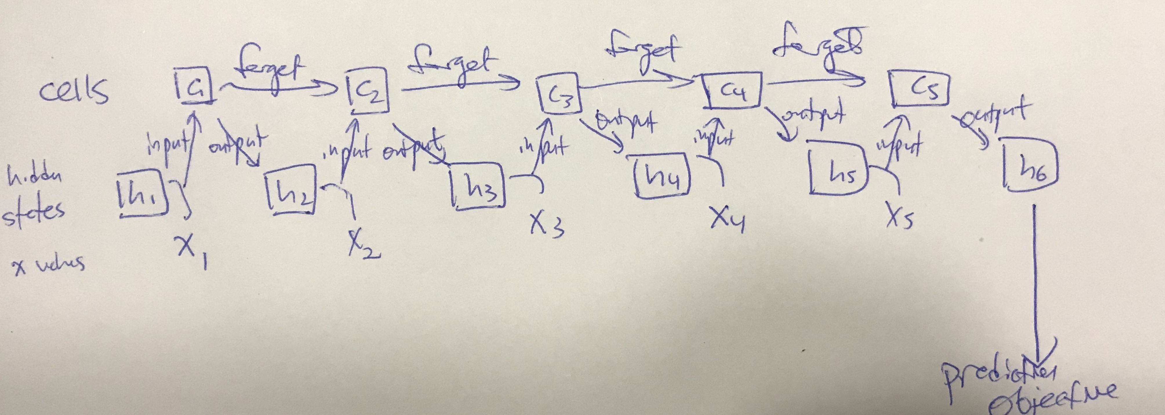
LSTM diagram
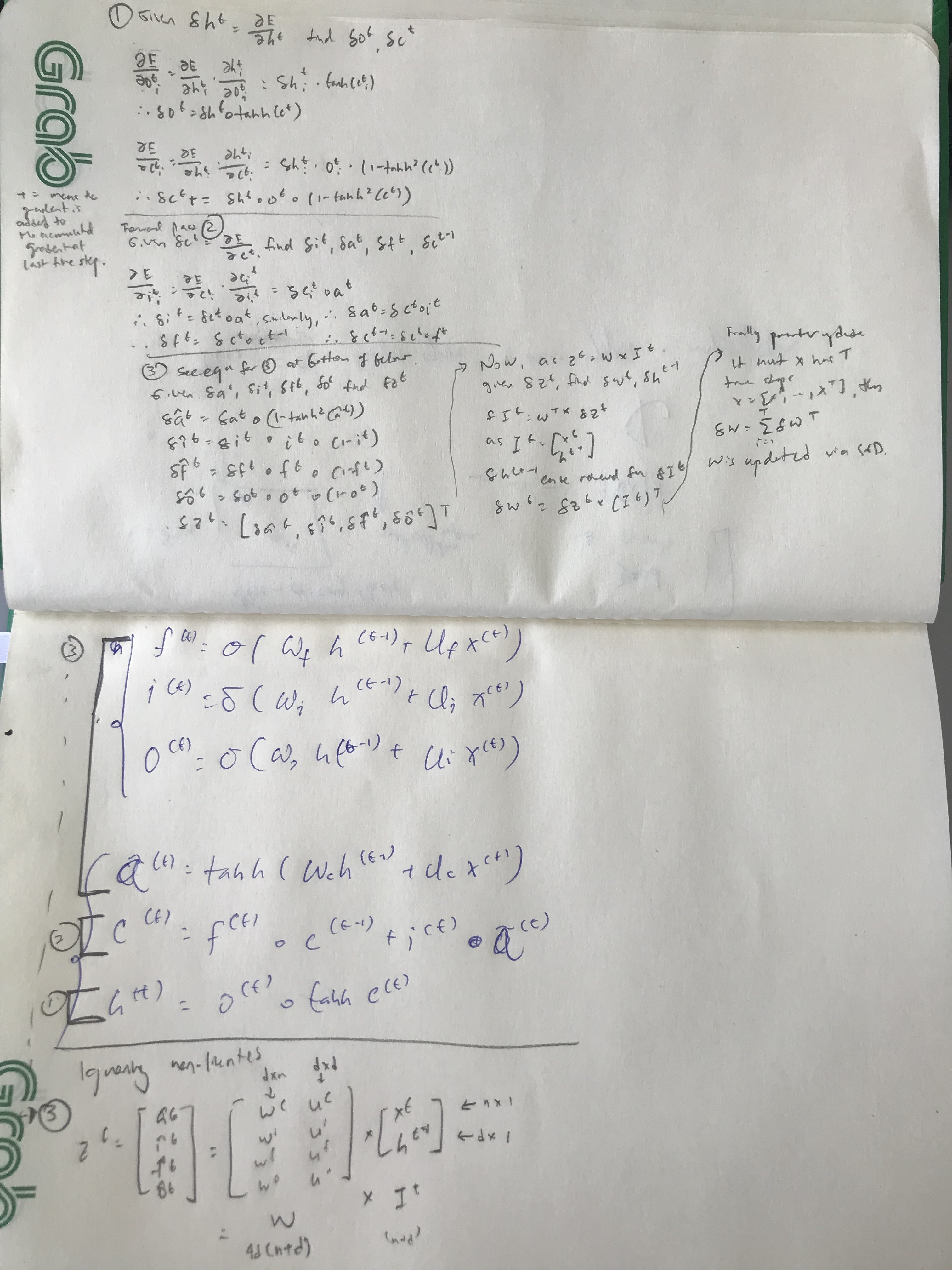
Walking through LSTM backdrop
** **
My thoughts on how RNNs work in general:
On my question about RNNs and the last hidden state of a decoder: No, there is no residual meaning. Let’s recall how the hidden state was formed. Recall that we have weights learned from applying millions of lines of parallel Eng-Fre data. These weights will take a sequence of English words and map them into the shared Eng-Fre embedding space. The embedding works by essentially pointing to one particular rotation on the 300-dim unit sphere [1], which is cared up into chunks corresponding to words in Eng (or Fre). The embedding has the properties that (a) it is closest in value (via dot-product) to the next word that it is supposed to output (if doing translation the next word is represented by the French word embeddings, but in language modeling or whatever the next word is the next likely word) and also (b) applying the RNN transformation on it (weight matrix plus input plus ReLU) changes the vector to point to the next word we want to decode (in a language model the input is the currently produced word).[2] But the training data never had any examples of anything following (EOS) so what we get if we apply the decoder transformation to the last hidden state was never learned and is simply random depending on our model initialisations.
[1] Technically they have a magnitude also but typically we normalize them so we can think of them on the unit sphere.
[2] Another way to say it is, you decode, the ‘signal’ of the word to be decoded is the largest in the hidden state (which is why when you dot product it with your vocab and take a softmax it pops up on top). [The interterpretation of a strong ’signal’ is precicely defined by ‘it is the closest to x vector out of all possible word vectors such that when you apply a softmax x pops out’) But there is also other underlying ‘signals’ about all the other words that you have encoded, only they are hidden in the background and will emerge when you apply your RNN transformation to it.
[3] By the way, the weight matrix multiplication is simply a rotation in 300 dimensional space. We need to have a non-linearity so that the rotation is not simply the same every time - then it would be impossible to also get the feature (1) of matching our word embeddings after every transformation!.
Some thoughts on the limitations of RNNs:
The probem with RNNs is not that their hidden state gets overwritten (the number of concepts you can store in a 300 dimensional vector is mind-blowingly large.) You have a 300 dim space, put in some vector that represents some word, transform it in some way, put in some other vector that represents some word… The non-linearity at each step allows us to jump around the space so that we can match different word embeddings. It’s not that the space is not big enough to store all possible sentences.
It’s that it’s hard to train. It’s a backprop problem, not a forward prop problem. And that is because model weights from far away get overwhelmed by model weights from close by. It can learn all close-by dependencies, but not far away dependencies.
How does the LSTM help
Walking through LSTM backdrop
Relative insensitivity to gap length is an advantage of LSTM over RNNs. How does it achieve this? The first thing to note is that the forget gate and input gate are mostly 1. Also, in an LSTM, the cell is the primary memory store, where the recurrence happens. Each hidden state is like a derivation of the cell state.
Then the LSTM cell is like an attention layer. At cell state c_5, it might contain selected parts from hidden states h_1, h_3, and h_4, depending on what it has chosen to forget. The subspaces of the cell state that are not forgotten are carried forward (identity) to the last cell state, so there is no loss of backprop signal. The LSTM learns (in its cell states) “what is the compilation of previous hidden states do I need to remember to generate the next output”?
The LSTM roughly captures: “Whenever I see a particular phrase or some linguistic phenomenon a, I must remember it and carry over its signal to where I will use it, and whenever I see somethign else b I will remember it, and when I see c, presumably I have used a and b and will forget them.
Another more convoluted way to put it is: The cell states are the ‘primary’ parts of the memory unit where the recurrence happens, the hidden states are reflections of the cell state. The cell state ‘accumulates’ information and passes it down to future cell states through the ‘Constant Error Carousel’, which is basically the forget gate. As the forget gate is usually 1 except for parts that are learned to be forgotten, the parts that are not forgotten are carried forward with no loss of signal on the backprop. (Indeed, vanilla LSTMs don’t have a forget gate and instead add an unchanged cell state (e.g. a recurrent connection with a constant weight of 1). This addition is called the Constant Error Carousel because it solves the training problem of vanishing and exploding gradients. )
Some notes about LSTM:
-
The forget gate is actually irrelevant and not very useful. To have a forget gate and an output gate is a bit overkill.
-
If you have vanishing gradients, any gradient g + 0 is still g, so you still retain the local updates. However, if gradients explode, all of them do. That is because some gradient g + infinity is infinity. That is the reason why LSTM does not protect you from exploding gradients, since LSTM also uses a recurrent weight matrix, not only internal state-to-state connections. So successful LSTM applications typically use gradient clipping.
-
Note that the forget gate in actuality is not always 1, and the amount of long0term information lost at each time step is the value of the forget gate. If the forget gate is close to 0, we get a vanilla RNN that loses long-term dependencies. So the forget gate must be well initialized.
-
LSTM training should be not too much slower than vanilla RNN training, because the complexity of the model increased in space, but the time compelxity is still a matmul (on a much bigger matrix, see the big W which captures the candidate cell state, and all three gates which can be all computed at once on my derivation pic above), some linearities, and a non-linearity.
What about GRUs
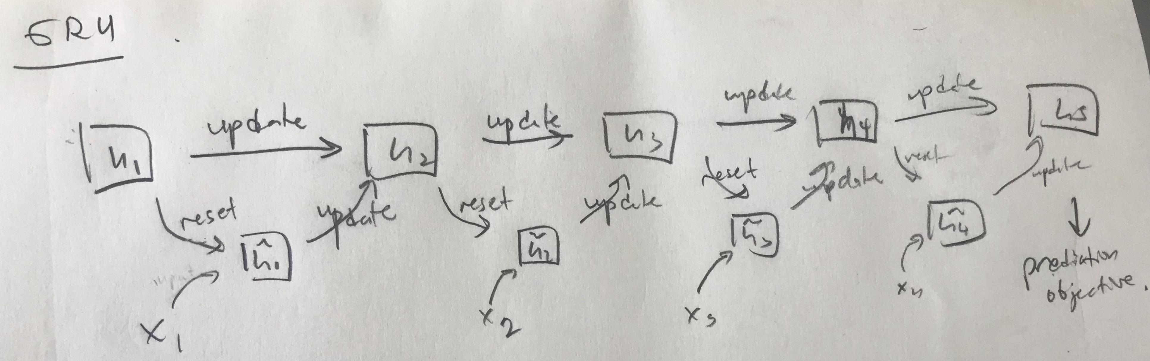 I said that the forget gate is actually unnecessary. The 300-dim space is enough to capture all saved concepts without ever needing to ‘forget’ them to ‘free up space’. In addition, it’s a bit cluttered to have a separate ‘cell’ and to have a hidden state as a derivation of the cell. We can just directly use the hidden state as the cell.
So, in the GRU equations
\begin{align}
\text{Update Gate (1)} && u^{(t)} = & \sigma(W_uh^{(t-1)} + U_u x^{(t)})
\text{Reset Gate (2)} && r^{(t)} = & \sigma(W_rh^{(t-1)} + U_r x^{(t)})
\text{New Hidden State Content (3)} && \tilde h^{(t)} = & \tanh(W_h(r^{(t)} \circ h^{(t-1)}) + U_h x^{(t)})
\text{Hidden State (4)} && h^{(t)} = & (1-u^{(t)}) \circ h^{(t-1)} + u^{(t)} \circ \tilde h^{(t)}
\end{align}
The key part of the GRU is the 4th equation, where some parts of the last hidden state are carried forward (letting us push backprop over logn-term info if the gates remain 1 over the time period of the dependency) and other parts are written over.
The 2nd equation above learns, for each hidden state and new content, what parts to write over to fit into a new subspace and not overwrite any previous content.
You may think, okay, the update gate in the GRU handles the input gate and the forget gate, and the reset gate handles the ourput gate in the LSTM. But why have a reset gate at all. Isn’t the forget gate (aka GRU update gate) enough to do all the updates? Who cares, becasue the subspace will not get that cluttered - it is huge - why do we need to overwrite any information as per reset gate anyways?
Indeed, this is true. Both Arxiv https://arxiv.org/pdf/1804.04849.pdf and Reddit https://www.reddit.com/r/MachineLearning/comments/7x72h6/d_why_reset_gate_in_gru/ Confirm that you can just have an LSTM/GRU with only a forget (GRU update) gate, and it will work great. So the reset gate is more for theoretical properties, not super important.
The wider implications of these thoughts to AI
AI models can learn not only representations of objects or states, but also of sequences of those objects or states, or to put it another way, a transformation that turns one object into the next. But sequences are vital to planning and decision-making. That process would include:
(1) Embedding of possible states of being into an embedding space
(2) Playing out most likely sequences of events (with e.g beam search), with the transition function learned from experience.
(3) Making decisions based on these sequences’ end states or side-effects given some reward function.
Where we are far away from AI currently is
(1) Capturing long-long-term dependency information (This must be stored somewhere in persistent memory and there must be some trigger to take it out when it is needed)
(2) Representing complex and compositional events or states or objects, and the interactions of events on objects.
-
Hierarchical/Compositional embedding is hard . In word vectors we just took words as tokens and threw them into the word2vec model, and the embeddings that came our corresponded to the simple couting relationships between words in text. But . It doesn’t really matter what the embedding is, if you get a hierarchical embedding you can train a transition function to match it. One important thing about the embedding is that the distinct entities must be far away angle-wise in 300 dimensional space.
-
For example, could we maybe some embeddings about entities always updated, and then somehow. We have some embedding for ‘Sally’, and we have some embedding for ‘sick person’ (or alternately, a transformaiton which corresponds to ‘has become sick’), and we apply it to Sally to get ‘Sick sally’. Then when Sally gets well, we invert the transformation (so the transformation to ‘get well’ must be the inverse of the one ‘to get sick’) to get back ‘Sally’. This is compositional embeddings.
These are like classes in object oriented programming.
We need to be able to define different ‘distance’ metrics between different classes. These distance metrics are probably goal-specific.
Idea: One can define one PARTICULAR invertible transformation ‘derivative’ in the 300 dimensional space, such that if one follows it one can arrive at
one can define two actually: ‘derive subclass’ and ‘derive attribute’
This has to be easy to compute such that all the deivatives can be computed rapidly and be gotten all at once (a brown cat is a mammal is an animal is a living being & is brown)
Now the last part is that there must be some way to learn new classes and new attributes of classes, after seeing them enough times, as well as the transformations that generate such attributes. The number of available transfomations to do this should be kept in a limited number and should be very easy to mark out and should not look like any other transformations (ie the transition functions between states over time - and its not physical time that matters but action time - time between events and interaction with other objects).
In other words, it seems like the attributes for ‘color’ must live in some subspace of the 300-d space, and the cat must be 18 x
There is some transform (has-attribute)
Presumably it is required to use a medium large embedding space that one can be confident of not using up (not too large or the model loses its grip and is ahrd to trian).
Knowing that millions of people around the world would be watching in person and on television and expecting great things from him and realizing that his legs could no longer carry him down the runway with the same blazing speed and confidence in making a huge, eye-popping leap that they were capable of a few years ago, the renowned sprinter and track-and-field personality Carl Lewis, made only a few appearances in races during the few months before the Summer Olympics in Atlanta, Georgia because he wanted to conserve his energies and concentrate on the job at hand.
One way (is there another?) is to have a dictionary of all the entities in the world and the states that can happen to them.
given an objective function.
LINGUSTICS ASIDE: In English, there are words that correspond to objects, and those are NOUNS (noun phrases). There are words that correspond to attributes, and those are ADJECTIVES (adjectival phrases). The point is: define some grammatical primitives like NOUNS and ADJECTIVES, restrict those to exist in only a subset of the embedding space, define some grammar rules as fixed transformations, ensure that the learned transformations will not overshadow these fixed transformations. The learned transformations are transitions from a composed embedding of an entity to another over (action) time (that is, with verbs), the fixed transformations are compositions of attributes to enrich the embeddings of the entities.
<The above must be trained on gramatically correct corpora, but if done so I believe it could build a knowledge bank or world knowledge>. I want to build a machine learned knowledge base.
** **
Appendices:** **
Appendix 1 Notes:
-
Why apply a tanh to the cell before applying an output gate, since it went through a tanh already? Not sure.
-
Why does forget gate only depend on h_t=1, not c_t-1? Becuase we don’t need to forget things stored in the cell - there is enough space in the 300 dimensional space to store whatever we want. We only forget if carrying over the signal is no longer necessary, and that depends on h_t=1.
-
Why so many gates? Isn’t it possible that they be way underspecified? (I suspect they did this to make the model theoretically as powerful as possible, but yes, it is underspecified and that’s why they invented GRUs).
-
Another random question: Do RNNs capture positional information (like this is the first word this is the second word this is the third word, etc?) It must but how? Is it just by how weak its signal is compared to more recent words? Is it (generally, I know that all trainings may have different results) put into different parts of the embedding space? (I think thats what it does actually. Idea: maybe each new word also writes a ‘pointer’ at the location of the last word to where it will write the new word).
Appendix 2: